Clustering

Load, filter, embed

import numpy as np
import scanpy as sc
import matplotlib.pyplot as plt

sc.settings.verbosity = 3
np.random.seed(42)

adata = sc.read_10x_mtx("/opt/data/pbmc3k", var_names="gene_symbols",
                        make_unique=True)
adata.layers["counts"] = adata.X.copy()
adata.var["mt"] = adata.var_names.str.startswith("MT-")
sc.pp.calculate_qc_metrics(adata, qc_vars=["mt"], percent_top=None,
                           log1p=False, inplace=True)


def is_outlier(adata, metric, nmads):
    """Flag cells whose metric sits more than nmads MADs from the median.

    Args:
        adata: AnnData object holding the metric in .obs.
        metric: Column of adata.obs to test.
        nmads: Number of median absolute deviations for the cutoff.

    Returns:
        Boolean Series, True where the cell is an outlier.
    """
    values = adata.obs[metric]
    median = values.median()
    mad = (values - median).abs().median()
    return (values < median - nmads * mad) | (values > median + nmads * mad)


adata.obs["log1p_total_counts"] = np.log1p(adata.obs["total_counts"])
adata.obs["log1p_n_genes_by_counts"] = np.log1p(
    adata.obs["n_genes_by_counts"]
)
adata.obs["outlier"] = (
    is_outlier(adata, "log1p_total_counts", 5)
    | is_outlier(adata, "log1p_n_genes_by_counts", 5)
    | is_outlier(adata, "pct_counts_mt", 3)
)
adata = adata[~adata.obs["outlier"]].copy()
sc.pp.filter_genes(adata, min_cells=3)

sc.pp.normalize_total(adata, target_sum=1e4)
sc.pp.log1p(adata)
sc.pp.highly_variable_genes(adata, layer="counts", n_top_genes=2000,
                            flavor="seurat_v3")
adata.raw = adata
adata = adata[:, adata.var["highly_variable"]]
sc.pp.scale(adata, max_value=10)
sc.tl.pca(adata, n_comps=50, random_state=42)
sc.pp.neighbors(adata, n_neighbors=15, n_pcs=30, random_state=42)
sc.tl.umap(adata, random_state=42)
print(adata.shape)

(2428, 2000)

Leiden clustering

# Leiden community detection on the KNN graph, the clustering
# sc-best-practices recommends. The igraph flavour is the current
# default backend.
sc.tl.leiden(adata, resolution=0.5, key_added="leiden", random_state=42,
             flavor="igraph", n_iterations=2, directed=False)

print(adata.obs["leiden"].value_counts().sort_index())

leiden
0    1099
1     456
2     412
3     315
4     146
Name: count, dtype: int64

sc.pl.umap(adata, color="leiden", show=False)
plt.savefig("outputs/clustering_leiden.png", dpi=150, bbox_inches="tight")
plt.close()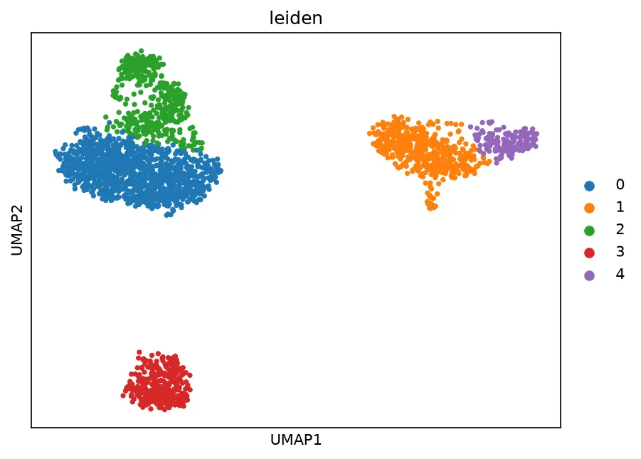

UMAP colored by the Leiden clusters at resolution 0.5. Seven clusters cover the embedding, with the large cluster on one arm and the smaller populations each holding their own region.

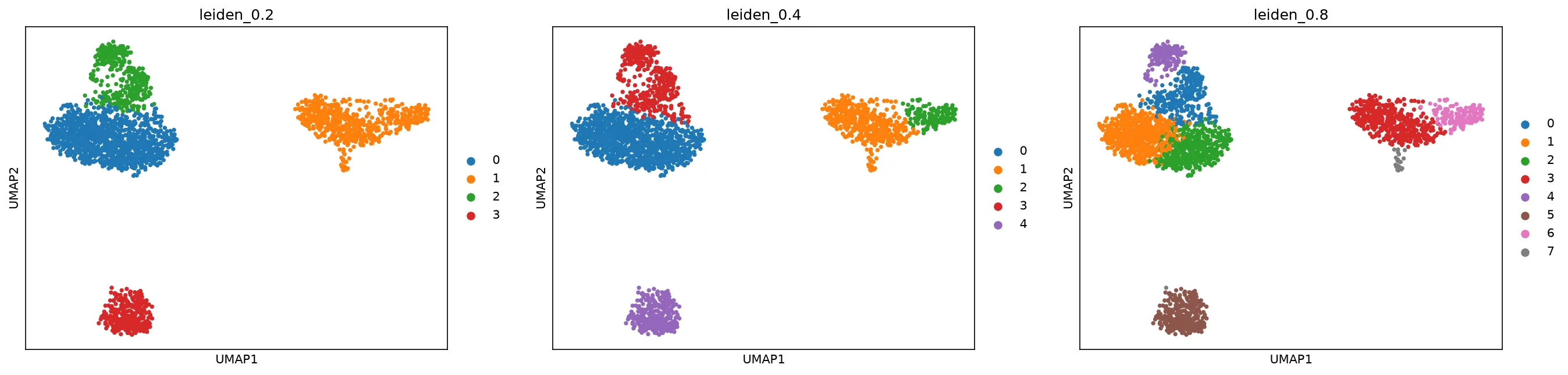
Testing resolutions

# Try multiple resolutions. Higher resolution splits more populations
# apart; sc-best-practices uses these sweeps to focus on
# substructures.
for resolution in (0.2, 0.4, 0.6, 0.8, 1.0):
    sc.tl.leiden(adata, resolution=resolution,
                 key_added=f"leiden_{resolution}", random_state=42,
                 flavor="igraph", n_iterations=2, directed=False)
    n_clusters = adata.obs[f"leiden_{resolution}"].nunique()
    print(f"resolution {resolution}: {n_clusters} clusters")

resolution 0.2: 4 clusters
resolution 0.4: 5 clusters
resolution 0.6: 6 clusters
resolution 0.8: 8 clusters
resolution 1.0: 8 clusters

Comparing the partitions

from sklearn.metrics import adjusted_rand_score

# The adjusted Rand index measures agreement between two partitions,
# corrected for chance. Agreement above 0.9 means the resolutions
# describe almost the same structure.
for resolution in (0.2, 0.4, 0.6, 0.8, 1.0):
    ari = adjusted_rand_score(adata.obs["leiden"],
                              adata.obs[f"leiden_{resolution}"])
    print(f"ARI of {resolution} against 0.5: {ari:.3f}")

ARI of 0.2 against 0.5: 0.889
ARI of 0.4 against 0.5: 0.990
ARI of 0.6 against 0.5: 0.987
ARI of 0.8 against 0.5: 0.656
ARI of 1.0 against 0.5: 0.653

sc.pl.umap(adata, color=["leiden_0.2", "leiden_0.4", "leiden_0.8"],
           show=False)
plt.savefig("outputs/clustering_resolutions.png", dpi=150,
            bbox_inches="tight")
plt.close()

UMAP at resolutions 0.2, 0.4 and 0.8 side by side. Resolution 0.2 merges the arms into four broad groups, 0.4 matches the seven clusters of 0.5, and 0.8 begins to split the largest arm.