Gene Set Enrichment Analysis

Differential expression analysis gives you a list of individual genes. But biology does not work one gene at a time. Genes act together in pathways and programs. A treatment might modestly change dozens of genes in the same pathway. None of those genes would pass a strict significance cutoff on their own. Yet the coordinated shift across the entire pathway is real and meaningful.

Gene Set Enrichment Analysis solves this problem. GSEA looks for coordinated changes across predefined groups of genes. It can detect subtle but consistent shifts that single gene analysis misses.

How GSEA works

GSEA starts with a ranked list of all genes. You rank them by some metric from your differential expression results. The Wald statistic from DESeq2 works well because it captures both the magnitude and certainty of change. Genes strongly upregulated by treatment go to the top. Genes strongly downregulated go to the bottom.

Next, GSEA takes a gene set. A gene set is a predefined list of genes that belong to a biological pathway or process. GSEA walks down your ranked list from top to bottom. Every time it hits a gene from the set, it takes a step up. Every time it hits a gene not in the set, it takes a step down. This produces a running enrichment score.

If genes in the set cluster near the top of the ranked list, the enrichment score swings strongly positive. If they cluster near the bottom, it swings strongly negative. If they are scattered randomly, the score stays near zero.

The Normalized Enrichment Score (NES) adjusts for gene set size. A positive NES means the pathway is enriched among upregulated genes. A negative NES means the pathway is enriched among downregulated genes. The adjusted p-value tells you whether the enrichment is statistically significant.

GSEA vs ORA

Over-Representation Analysis is the other common approach to pathway analysis. The key difference is the input.

Feature	GSEA	ORA
Input	All genes, ranked by a metric	Only significant genes above a cutoff
Cutoff needed	No	Yes
Uses fold change information	Yes	No
Detects subtle coordinated changes	Yes	No

GSEA uses every gene in your dataset. It does not require an arbitrary significance cutoff. ORA throws away all non-significant genes and only asks whether significant genes are overrepresented in certain pathways. This means ORA loses information. GSEA is generally preferred when you have genome-wide results from a differential expression analysis.

Setup

We use the fgsea package for the analysis and MSigDB Hallmark gene sets. The Hallmark collection contains 50 well-defined biological pathways. These are curated to reduce redundancy and noise.

library(tidyverse)
library(fgsea)
library(msigdbr)

The DESeq2 result

The page recomputes the differential expression so it stands on its own. Each row has a gene, a test statistic and a p-value, and the statistic is what the ranking uses.

library(DESeq2)
library(airway)

data("airway")
dds <- DESeqDataSet(airway, design = ~ cell + dex)
dds$dex <- relevel(dds$dex, ref = "untrt")
dds <- dds[rowSums(counts(dds)) >= 10, ]
dds <- DESeq(dds)

res <- as.data.frame(results(dds, contrast = c("dex", "trt", "untrt")))
res$gene <- rownames(res)
nrow(res)

[1] 22369

Create the ranked gene list

GSEA needs a named numeric vector. The names are gene IDs. The values are the ranking metric. We use the stat column from DESeq2. This is the Wald test statistic. It captures both effect size and precision in a single number.

ranks <- res |>
  filter(!is.na(stat)) |>
  arrange(desc(stat)) |>
  pull(stat, name = gene)

length(ranks)

[1] 22369

The top genes have the largest positive statistics. These are the most strongly upregulated genes. The bottom genes have the most negative statistics.

head(ranks, 5)

ENSG00000152583 ENSG00000165995 ENSG00000120129 ENSG00000101347 ENSG00000189221
       24.83137        24.73530        24.18720        24.14882        23.58722

tail(ranks, 5)

ENSG00000146250 ENSG00000107562 ENSG00000148848 ENSG00000178695 ENSG00000162692
      -17.83889       -17.98509       -18.00964       -18.74979       -19.42798

Get Hallmark gene sets

We use the msigdbr package to download MSigDB Hallmark gene sets. These are formatted as Ensembl gene IDs to match our DESeq2 results.

# msigdbr renamed the argument from category to collection in version 10.
hallmark <- msigdbr(species = "Homo sapiens", collection = "H") |>
  dplyr::select(gs_name, ensembl_gene)

# Convert to the list format fgsea expects
pathways <- hallmark |>
  group_by(gs_name) |>
  summarise(genes = list(ensembl_gene)) |>
  deframe()

length(pathways)

# Hand the ranking and the same 50 sets to the Python tab.
dir.create("outputs", showWarnings = FALSE, recursive = TRUE)
write_csv(
  tibble(gene = names(ranks), stat = as.numeric(ranks)),
  "outputs/gsea_ranks.csv"
)
write_csv(hallmark, "outputs/gsea_hallmark.csv")

[1] 50

We have 50 Hallmark pathways ready for testing.

Run fgsea

The fgsea() function performs the enrichment analysis. We set a minimum gene set size of 15 and a maximum of 500 to avoid testing very small or very large sets.

set.seed(42)
gsea_res <- fgsea(
  pathways = pathways,
  stats = ranks,
  minSize = 15,
  maxSize = 500
)

gsea_res <- gsea_res |>
  as_tibble() |>
  arrange(padj)

Interpret the results

Let’s look at the top 10 enriched pathways.

gsea_res |>
  dplyr::select(pathway, pval, padj, NES, size) |>
  head(10)

# A tibble: 10 × 5
   pathway                                     pval        padj   NES  size
   <chr>                                      <dbl>       <dbl> <dbl> <int>
 1 HALLMARK_ADIPOGENESIS              0.00000000246 0.000000123  2.05   193
 2 HALLMARK_TNFA_SIGNALING_VIA_NFKB   0.00000337    0.0000842    1.85   184
 3 HALLMARK_OXIDATIVE_PHOSPHORYLATION 0.0000295     0.000492     1.70   200
 4 HALLMARK_ANDROGEN_RESPONSE         0.000408      0.00396      1.77    92
 5 HALLMARK_COMPLEMENT                0.000554      0.00396      1.62   160
 6 HALLMARK_E2F_TARGETS               0.000488      0.00396     -1.52   200
 7 HALLMARK_P53_PATHWAY               0.000347      0.00396     -1.57   187
 8 HALLMARK_FATTY_ACID_METABOLISM     0.00106       0.00443      1.60   144
 9 HALLMARK_IL2_STAT5_SIGNALING       0.000869      0.00443      1.58   175
10 HALLMARK_MTORC1_SIGNALING          0.000826      0.00443     -1.48   196

The NES column tells the story. Adipogenesis has the highest NES at 2.05. This means genes in the adipogenesis pathway are strongly enriched among genes upregulated by dexamethasone treatment. This makes biological sense. Dexamethasone is a glucocorticoid that promotes fat cell differentiation.

TNF-alpha signaling via NF-kB is the second most enriched pathway. Glucocorticoids are well known anti-inflammatory agents that interact with the NF-kB pathway.

The P53 pathway has a negative NES of -1.57. This means P53 pathway genes tend to be downregulated by treatment.

Overall, 16 pathways are significantly enriched among upregulated genes and 6 among downregulated genes.

gsea_res |>
  filter(padj < 0.05) |>
  dplyr::count(direction = ifelse(NES > 0, "up", "down"))

# A tibble: 2 × 2
  direction     n
  <chr>     <int>
1 down          6
2 up           16

NES bar chart

A bar chart of NES values gives a quick overview of all significant pathways. Bars pointing right are upregulated pathways. Bars pointing left are downregulated.

nes_plot <- gsea_res |>
  filter(padj < 0.05) |>
  mutate(
    pathway = str_remove(pathway, "HALLMARK_") |>
      str_replace_all("_", " ") |>
      str_to_title(),
    pathway = fct_reorder(pathway, NES)
  ) |>
  ggplot(aes(x = NES, y = pathway, fill = NES > 0)) +
  geom_col() +
  scale_fill_manual(values = c("TRUE" = "#E74C3C", "FALSE" = "#3498DB")) +
  labs(x = "Normalized Enrichment Score", y = NULL) +
  theme_minimal() +
  theme(legend.position = "none")

ggsave("outputs/gsea-barplot.png", nes_plot,
       width = 8, height = 6, dpi = 110, bg = "white")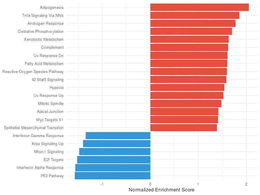

The chart clearly separates pathways activated by dexamethasone from those suppressed. Adipogenesis, androgen response, and TNF-alpha signaling are the most strongly upregulated. E2F targets, G2M checkpoint, and P53 pathway are among the downregulated pathways.

Enrichment plot

The enrichment plot shows the running enrichment score for a single pathway. It reveals where in the ranked list the pathway genes are concentrated.

top_pathway <- gsea_res$pathway[1]

enrichment_plot <- plotEnrichment(pathways[[top_pathway]], ranks) +
  labs(title = top_pathway) +
  theme_minimal()

ggsave("outputs/gsea-enrichment.png", enrichment_plot,
       width = 7, height = 4, dpi = 110, bg = "white")
top_pathway

[1] "HALLMARK_ADIPOGENESIS"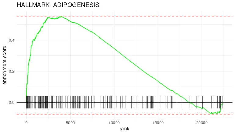

The green line rises steeply at the left side of the plot. This means adipogenesis genes are concentrated among the most upregulated genes. The vertical black lines at the bottom show where each pathway gene falls in the ranked list. Most cluster toward the left.

Export results

Save the full GSEA results for downstream use.

gsea_res |>
  dplyr::select(-leadingEdge) |>
  write_csv("outputs/gsea_results.csv")

The same test in Python

gseapy.prerank runs the same algorithm on the ranking and the sets exported above, so the two tabs are comparing implementations rather than inputs.

Python

import pandas as pd
import gseapy as gp

ranks = pd.read_csv("outputs/gsea_ranks.csv").set_index("gene")["stat"]
hallmark = pd.read_csv("outputs/gsea_hallmark.csv")
gene_sets = hallmark.groupby("gs_name")["ensembl_gene"].apply(list).to_dict()

pre_res = gp.prerank(
    rnk=ranks,
    gene_sets=gene_sets,
    permutation_num=1000,
    min_size=15,
    max_size=500,
    seed=42,
    outdir=None,
)

results = pre_res.res2d.copy()
results["FDR q-val"] = pd.to_numeric(results["FDR q-val"])
results = results.sort_values("FDR q-val")
columns = ["Term", "NES", "FDR q-val"]
print(len(results))
print(results[columns].head(10).to_string(index=False))

50
                                    Term       NES  FDR q-val
                   HALLMARK_ADIPOGENESIS  2.037564   0.000000
        HALLMARK_TNFA_SIGNALING_VIA_NFKB  1.857868   0.004034
              HALLMARK_ANDROGEN_RESPONSE  1.774583   0.006147
      HALLMARK_OXIDATIVE_PHOSPHORYLATION  1.689226   0.013831
          HALLMARK_FATTY_ACID_METABOLISM  1.609689   0.015560
                 HALLMARK_UV_RESPONSE_DN  1.603783   0.015624
          HALLMARK_XENOBIOTIC_METABOLISM    1.6443   0.015905
                     HALLMARK_COMPLEMENT  1.615163   0.017124
HALLMARK_REACTIVE_OXYGEN_SPECIES_PATHWAY   1.62378   0.017865
            HALLMARK_IL2_STAT5_SIGNALING  1.566191   0.021207

Summary

GSEA detects coordinated expression changes across biological pathways. It uses all genes in your dataset and does not require a significance cutoff. In the airway dataset, GSEA found 22 significant Hallmark pathways. Most align with known glucocorticoid biology: adipogenesis, anti-inflammatory signaling, and metabolic regulation.