EDA for ML

Exploratory data analysis is the first step before building any model. You need to understand the shape of your data before choosing algorithms and preprocessing. Skipping it leads to poor models and wasted time. This page uses a synthetic classification dataset; the same patterns apply to any tabular data.

Every code block runs in a container in the companion repository, so the numbers and figure are real.

Load the data

from sklearn.datasets import make_classification

X, y = make_classification(n_samples=1000, n_features=10, n_informative=5,
                           n_redundant=2, weights=[0.85, 0.15], random_state=42)
df = pd.DataFrame(X, columns=[f"feature_{i}" for i in range(10)])
df["target"] = y
print(df.shape)

(1000, 11)

Target distribution

The first thing to check is the target. For classification, this reveals class imbalance.

df["target"].value_counts(normalize=True)

target
0    0.846
1    0.154

This 85/15 split matters: a model that always predicts class 0 scores 85% accuracy without learning anything, accuracy becomes misleading, and the minority class is usually the one you care about (disease positive). For regression, plot the target histogram and check for skew; a heavily skewed target may benefit from a log transform.

Missing values

missing = df.isnull().sum()
print((missing / len(df) * 100).round(1)[missing > 0])

Rules of thumb: under 5% missing, simple imputation is fine; 5 to 30%, consider whether missingness is informative; over 30%, consider dropping the column or adding a “was-missing” indicator.

Descriptive statistics

df.describe().round(2)

Look for scale differences (which demand scaling), unusual min/max values (possible outliers or errors), and near-zero standard deviations (features that carry no information).

Correlations

Highly correlated features are redundant. Tree models handle them fine; linear models can produce unstable coefficients.

corr = df.drop(columns=["target"]).corr()
# report pairs with |r| > 0.8

Highly correlated pairs (|r| > 0.8): none

No pairs cross 0.8 here. Real biological data often has correlated features (genes in a pathway co-express). When two features are highly correlated, drop one, combine them, or leave them if you use tree-based models.

Which features separate the classes?

df.groupby("target").mean().round(2)

        feature_0  feature_1  feature_2  feature_3  feature_4
target
0           -0.05      -0.04      -0.08      -1.03       0.94
1            1.07       0.14      -0.01      -0.09       0.16

Features whose means differ between classes carry signal. feature_0 goes from -0.05 to 1.07 across the classes; feature_3 from -1.03 to -0.09. A per-feature histogram colored by class makes this visual.

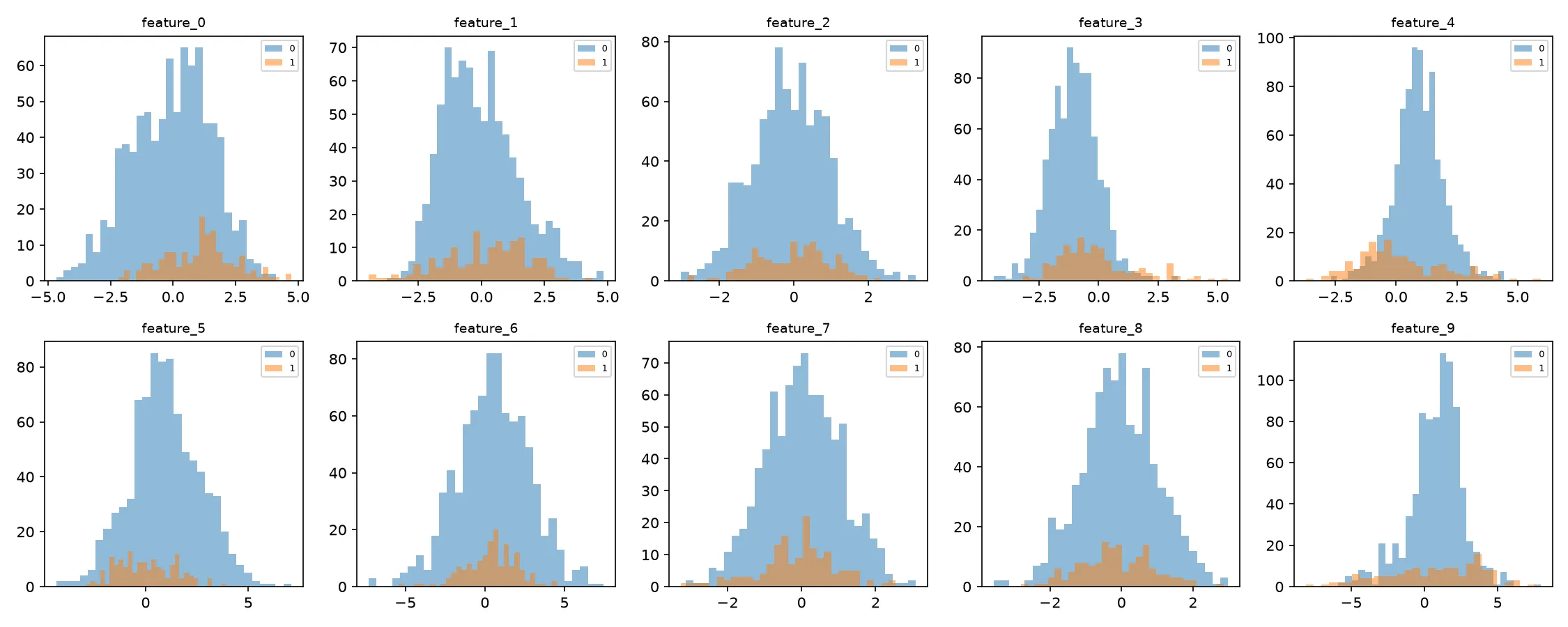
Features whose two histograms overlap heavily are less useful than those where the classes separate.

Outliers

from scipy import stats

z = np.abs(stats.zscore(df.drop(columns=["target"])))
print((z > 3).sum())

feature_3    16
feature_9    10
feature_4     6
...

A handful of outliers per feature is normal for 1000 samples. feature_3 has 16, worth a look. Options: cap at a percentile, remove if they are errors, transform to reduce skew, or do nothing (tree models are robust).

Duplicates

print(f"Duplicate rows: {df.duplicated().sum()}")

Duplicate rows: 0

A duplicate that lands in both train and test causes leakage. Deduplicate before splitting.

Checklist

Question	Check
How large is the dataset?	df.shape
Is the target balanced?	value_counts(normalize=True)
Missing values?	df.isnull().sum()
Feature scales similar?	df.describe()
Highly correlated features?	correlation matrix, threshold 0.8
Which features separate classes?	group by target, compare means
Outliers?	z-scores or IQR
Duplicates?	df.duplicated().sum()

Next steps

Now that you understand the data, the next page covers Preprocessing & Data Leakage, where you prepare it for modeling without leaking information.