Cox Proportional Hazards

The Kaplan-Meier curve compares whole groups. To adjust for covariates, and to put a number on a continuous predictor’s effect on survival, you need a model. Cox proportional hazards regression is that model, and its output, the hazard ratio, is the standard effect measure in survival studies. This page models survival on a treatment arm and a biomarker, in R and Python.

Every code block on this page runs in a container in the companion repository. The numbers and figure come from those real runs.

When to use Cox regression

Use it for time-to-event data when you want the effect of one or more covariates, adjusted for the others, without assuming a baseline survival shape. It reports a hazard ratio per covariate: the multiplicative change in the instantaneous risk.

The data

cox_data.csv has 150 patients with a survival time, an event flag, a treatment group, and a continuous biomarker.

library(survival)

df <- read.csv("cox_data.csv")
df$group <- factor(df$group, labels = c("control", "treated"))
fit <- coxph(Surv(time, event) ~ group + biomarker, data = df)
summary(fit)

                coef exp(coef) se(coef)      z Pr(>|z|)
grouptreated -1.0750    0.3413   0.1888 -5.693 1.25e-08 ***
biomarker     0.4473    1.5641   0.1102  4.059 4.92e-05 ***

             exp(coef) exp(-coef) lower .95 upper .95
grouptreated    0.3413     2.9301    0.2357    0.4941
biomarker       1.5641     0.6394    1.2603    1.9411
Concordance= 0.664

import pandas as pd
from lifelines import CoxPHFitter

df = pd.read_csv("cox_data.csv")
cph = CoxPHFitter()
cph.fit(df[["time", "event", "group", "biomarker"]],
        duration_col="time", event_col="event")
cph.print_summary()

           coef  exp(coef)  se(coef)  exp(coef) lower 95%  exp(coef) upper 95%      z       p
group     -1.08       0.34      0.19                 0.24                 0.49  -5.69  <0.005
biomarker  0.45       1.56      0.11                 1.26                 1.94   4.06  <0.005
Concordance = 0.66

Reading hazard ratios

The hazard ratio is exp(coef), and 1 is the no-effect line.

Treatment, HR 0.34. Treated patients have about a third of the hazard of controls at any moment. The confidence interval, 0.24 to 0.49, sits entirely below 1, so treatment is protective.
Biomarker, HR 1.56. Each one-unit rise in the biomarker raises the hazard by about 56%. Its interval, 1.26 to 1.94, sits above 1, so higher values are harmful.

A forest plot shows both at a glance, on a log scale, with the no-effect line at 1.

R
Python

library(broom)

td <- tidy(fit, exponentiate = TRUE, conf.int = TRUE)
ggplot(td, aes(estimate, term)) +
  geom_vline(xintercept = 1, linetype = "dashed") +
  geom_point() +
  geom_errorbarh(aes(xmin = conf.low, xmax = conf.high)) +
  scale_x_log10()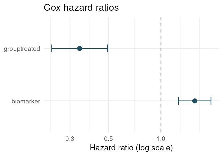

Forest plot of Cox hazard ratios (R)

import numpy as np

hr = np.exp(cph.params_)
ci = np.exp(cph.confidence_intervals_)
# plot hr with error bars on a log x-axis, vertical line at 1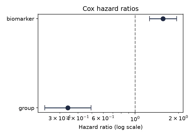

Forest plot of Cox hazard ratios (Python)

The proportional hazards assumption

Cox assumes each hazard ratio is constant over time. That is the one assumption you must check. Both languages test it from the scaled residuals.

R
Python

cox.zph(fit)

          chisq df     p
group     0.772  1 0.380
biomarker 5.161  1 0.023
GLOBAL    5.354  2 0.069

cph.check_assumptions(df[["time", "event", "group", "biomarker"]])

Proportional hazard assumption looks okay.

The global test is not significant (p = 0.069), so overall the assumption holds. R’s per-covariate test flags the biomarker as borderline (p = 0.023), a hint that its effect may drift over time. Worth a look, not a crisis.

Pitfalls and bioinformatics notes

Check proportional hazards. A crossing Kaplan-Meier plot or a significant cox.zph means the constant-hazard-ratio assumption is broken. Consider a time-varying effect or a stratified model.
A hazard ratio is relative. HR 0.34 means one third the risk, not one third the survival time. It says nothing about absolute benefit.
Enough events, not just patients. Cox power comes from events. A rough rule is ten events per covariate.
Standardize continuous covariates. A hazard ratio per raw unit can be tiny or huge depending on the scale. Report it per standard deviation or per clinically meaningful unit.

Key points

Cox regression models the hazard as a function of covariates and reports hazard ratios.
HR below 1 is protective, above 1 is harmful; the confidence interval versus 1 sets significance.
Always check the proportional-hazards assumption with cox.zph or check_assumptions.
R and Python give matching coefficients and hazard ratios.