MOFA: Unsupervised Factors

MOFA is PCA’s answer to multi-omics. It takes several data layers measured on the same samples and decomposes them into a handful of latent factors, where each factor is an axis of variation that can run through one layer or through several at once. Nobody tells it what to look for. It reads the four CLL layers and returns the directions along which patients differ most.

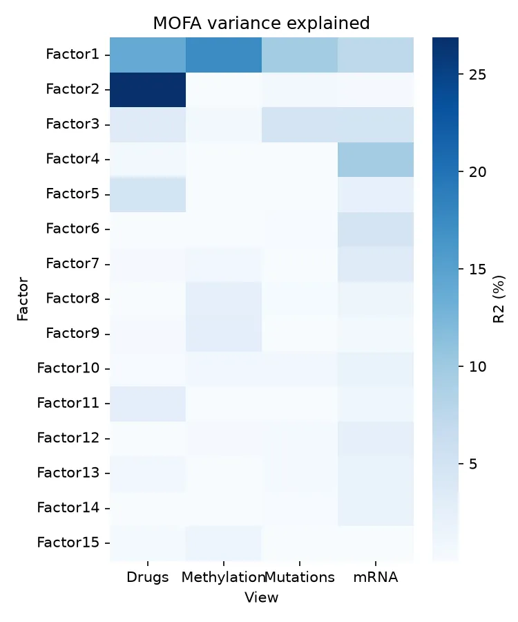
The output that matters is the variance each factor explains in each view. A factor that lights up in all four views is shared biology. A factor confined to one view is either view-specific signal or a technical artifact in that layer. That single table is what makes MOFA interpretable.

How it works

MOFA models each view as a product of a shared factor matrix and view-specific weights, Y_m ≈ Z Wᵀ_m, fitted in a Bayesian framework that shrinks unused factors toward zero. Two properties make it the first method to reach for. It handles missing values natively, so a patient absent from one layer still contributes through the others, and it separates variance per factor per view, so you can read straight off the result whether a factor is shared or private to one layer.

Both languages here run in the pinned multi-omics container. R trains the model with MOFA2; Python reads the same model file with mofax. The CLL data comes from the MOFAdata package inside the container, so nothing is downloaded by hand.

The data

Four views on 200 patients: drug response (310), methylation (4248 CpGs), mRNA (5000 genes), and mutations (69). MOFA needs no filtering to complete cases, which is part of the point. The model is given all 200 patients and left to handle the gaps.

R

Train the model, then read the variance decomposition and test each factor against IGHV status.

library(MOFA2)
library(MOFAdata)
data("CLL_data")                       # list of 4 matrices, features x 200 patients

mofa <- create_mofa(CLL_data)
model_opts <- get_default_model_options(mofa)
model_opts$num_factors <- 15           # a ceiling; unused factors shrink away
train_opts <- get_default_training_options(mofa)
train_opts$convergence_mode <- "slow"
train_opts$seed <- 42

mofa <- prepare_mofa(mofa, model_options = model_opts, training_options = train_opts)
mofa <- run_mofa(mofa, outfile = "CLL_model.hdf5", use_basilisk = FALSE)

The variance explained per factor per view is the map of the whole model. Factor 1 is the only factor with real weight in all four layers.

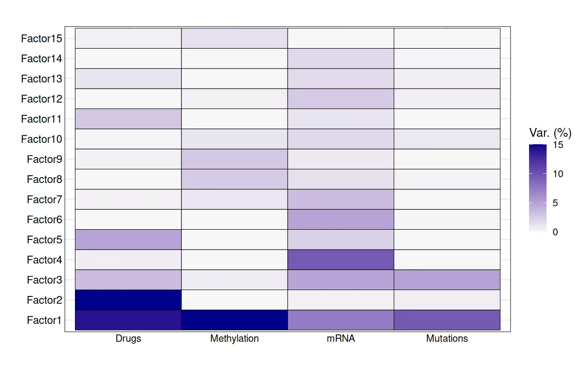
Across the whole model the layers give up different amounts of their variance: drugs 50.9%, mRNA 42.9%, methylation 26.9%, mutations 17.7%. Plotting the first four factors against IGHV status shows Factor 1 splitting the two subtypes cleanly while the others do not.

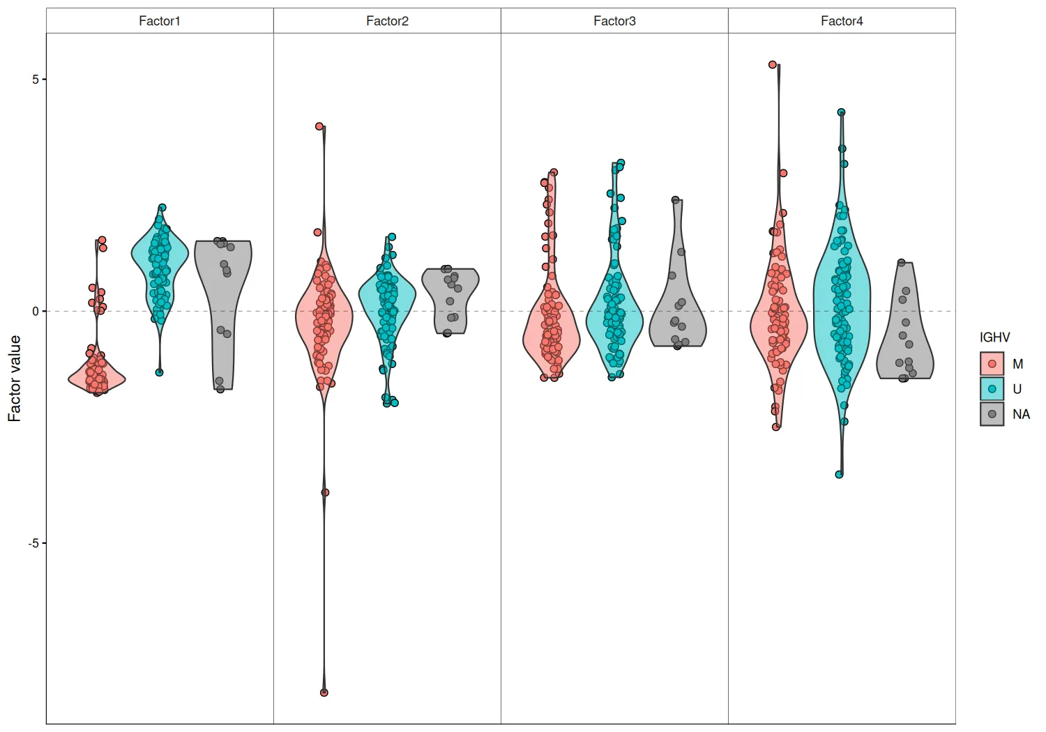
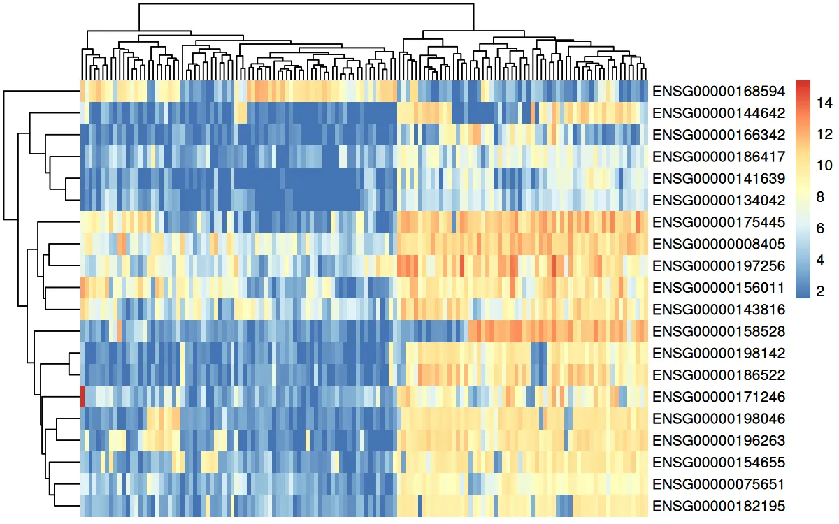
A Wilcoxon test confirms it. Factor 1 tracks IGHV at p = 4.97e-28; the next strongest, Factor 2, is five orders of magnitude weaker. To name Factor 1, read its top weights and the underlying data ordered by the factor.

plot_top_weights(model, view = "mRNA", factor = 1, nfeatures = 15)
plot_data_heatmap(model, view = "mRNA", factor = 1, features = 20, dendrogram = "both")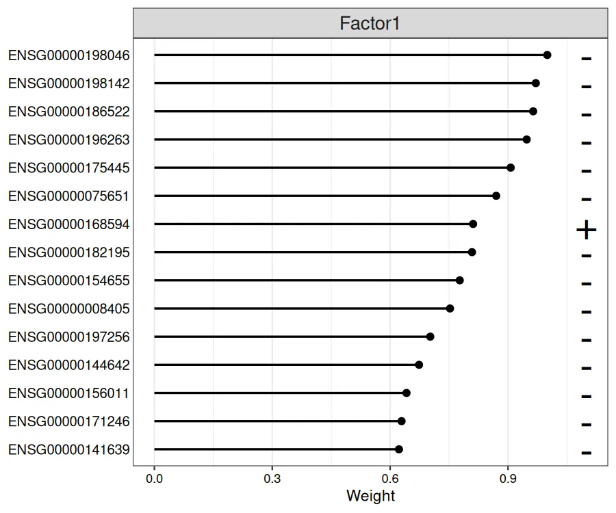

Python

A MOFA model is an HDF5 file, not an R object, so Python reads the exact model R trained. mofax is the companion package for that. This is not a re-fit: the factors and variance are the same numbers, which is the point worth showing.

import mofax as mfx

m = mfx.mofa_model("CLL_model.hdf5")
r2 = m.get_r2()                        # variance explained, per factor per view
factors = m.get_factors(factors=[0], df=True)   # Factor 1 values, indexed by sample

The variance heatmap is the same object the R plot draws, read from the same file.

IGHV is not stored as metadata, so pull it from the Mutations view. MOFA stores that view centered, so the two classes appear as one negative and one positive value; map by sign, then test Factor 1 against it.

import pandas as pd
from scipy.stats import mannwhitneyu

raw = m.get_data(views="Mutations", features=["IGHV"], df=True)["IGHV"]
ighv = pd.Series(pd.NA, index=raw.index, dtype=object)
ighv[raw > 0] = "U"
ighv[raw < 0] = "M"

df = factors.join(ighv.rename("IGHV")).dropna(subset=["IGHV"])
p = mannwhitneyu(df.loc[df.IGHV == "U", "Factor1"],
                 df.loc[df.IGHV == "M", "Factor1"]).pvalue   # 4.97e-28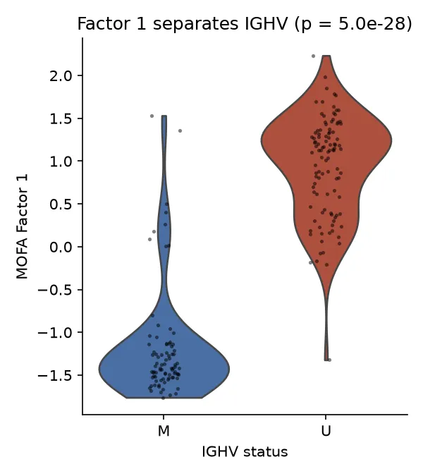

The Mann-Whitney p on the Python side is 4.97e-28 at n = 188, the same value the R Wilcoxon returns. Two languages, one model, one number. The model is portable; the analysis follows it.

What Factor 1 is

Factor 1 is the IGHV axis. IGHV mutation status is the strongest prognostic marker in CLL, and MOFA recovers it without ever being told it exists, from the joint structure of drug response, methylation, expression, and mutations. That it appears in all four views is the evidence that the split is real biology rather than a quirk of one assay. The remaining factors carry secondary structure: some are view-specific, like the mRNA-only Factor 4, and pick up variation that lives in a single layer.

Where MOFA stops

MOFA finds axes of variation, not clusters and not a classifier. If you need discrete patient subtypes, take the factors into a clustering step or use SNF. If you have a label and want a feature panel that predicts it, MOFA is the wrong tool and DIABLO is the right one. Watch the variance table for factors that correlate with the total number of detected features per sample: those often signal a normalization problem in one layer rather than biology, and MOFA will flag them in its own quality-control warnings.

The training script, the Python exploration, and the container are in the companion code repo under guides/multi-omics/mofa/.