Sample Size & Power

The most useful statistics happen before the experiment. A power analysis answers a simple question: how many samples do I need to detect an effect if it is real? Run it while you can still change the design, not after the data is in. This page does a power analysis for a two-sample comparison, in R and Python.

Every code block on this page runs in a container in the companion repository. The numbers and figure come from those real runs.

When to do a power analysis

Before you collect data. An underpowered study wastes samples and money, and it misses real effects. An overpowered one wastes the same resources chasing effects too small to matter. A power analysis picks the sample size that gives you a fair chance of finding an effect worth finding.

The four quantities

Power analysis ties together four numbers. Fix any three and the fourth is determined.

• Effect size. How large the difference is, in standard deviations. Cohen’s d of 0.2 is small, 0.5 is medium, 0.8 is large.
• Significance level (alpha). The false-positive rate, usually 0.05.
• Power. The chance of detecting a real effect, usually set to 0.80.
• Sample size. The number per group.

Power of a design

Given a design, how likely are we to detect the effect? Here we ask the power of a two-sample t-test with 20 samples per group and a large effect (d = 0.8).

R

power.t.test(n = 20, delta = 0.8, sd = 1, sig.level = 0.05, type = "two.sample")

     Two-sample t test power calculation

              n = 20
          delta = 0.8
             sd = 1
      sig.level = 0.05
          power = 0.6933994
    alternative = two.sided

Python

from statsmodels.stats.power import TTestIndPower

analysis = TTestIndPower()
analysis.power(effect_size=0.8, nobs1=20, alpha=0.05, ratio=1.0)

power at n=20, d=0.8: 0.693

Both languages agree: 20 per group gives only 69% power. That is below the usual 80% target, so this design would miss a real effect almost a third of the time.

Sample size for a target power

Turn the question around. How many samples per group do we need for 80% power?

R

power.t.test(power = 0.80, delta = 0.8, sd = 1, sig.level = 0.05, type = "two.sample")

              n = 25.52463
          delta = 0.8
          power = 0.8

Python

analysis.solve_power(effect_size=0.8, power=0.80, alpha=0.05, ratio=1.0)

n per group for 80% power, d=0.8: 25.5

Both give 25.5, so round up to 26 per group. Even a large effect needs more samples than people expect.

The power curve

A power curve shows how power grows with sample size, for several effect sizes at once. It makes the trade-off visible: smaller effects need many more samples.

R

ns <- 5:60
grid <- do.call(rbind, lapply(c(0.5, 0.8, 1.2), function(d) {
  pw <- sapply(ns, function(n) power.t.test(n = n, delta = d, sd = 1)$power)
  data.frame(n = ns, power = pw, d = factor(d))
}))

ggplot(grid, aes(n, power, color = d)) +
  geom_line(linewidth = 1) +
  geom_hline(yintercept = 0.8, linetype = "dashed")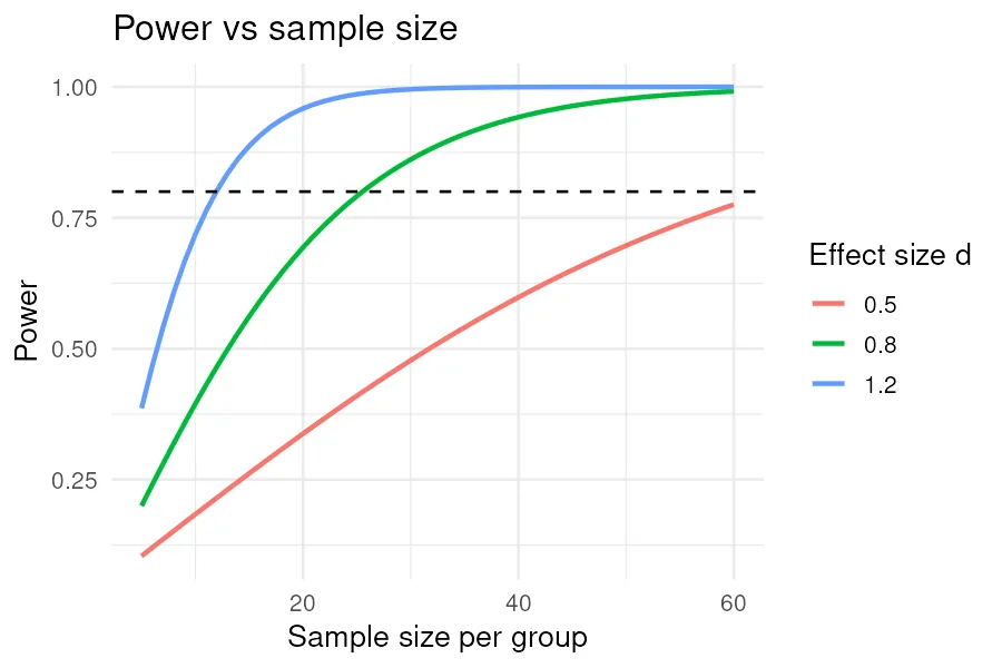

Python

import numpy as np

ns = np.arange(5, 61)
for d in [0.5, 0.8, 1.2]:
    plt.plot(ns, analysis.power(effect_size=d, nobs1=ns, alpha=0.05), label=f"d = {d}")
plt.axhline(0.8, ls="--", color="gray")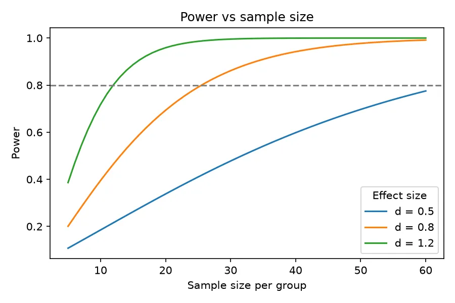

The large effect (d = 1.2) reaches 80% power by about 12 per group. The medium effect (d = 0.8) needs about 26. The small effect (d = 0.5) needs more than 60. Halving the effect size roughly quadruples the samples required.

Choosing an effect size

The effect size is the hard part, because it is the one number you do not yet know. Three honest ways to set it:

• Smallest effect of interest. Pick the smallest difference that would change a decision, and power for that. This is the most defensible choice.
• Pilot data. Estimate the effect from a small preliminary experiment, but treat it with caution, since small pilots are noisy.
• Published work. Borrow an effect size from a similar study, adjusting down, as published effects tend to be optimistic.

Pitfalls and bioinformatics notes

• Post-hoc power is misleading. Computing power from the effect you observed adds nothing beyond the p-value. Power analysis belongs before the study.
• Genomics multiplies the sample cost. Testing thousands of genes forces a much stricter alpha after multiple-testing correction, which raises the sample size needed per gene. See the Multiple testing guide.
• Design drives power too. Paired designs and covariate adjustment reduce noise and can lift power more than adding samples.

Key points

• Power analysis links effect size, alpha, power, and sample size. Fix three, solve for the fourth.
• Aim for 80% power at the smallest effect worth detecting.
• Smaller effects need dramatically more samples.
• Do the analysis before collecting data, never after.

Further reading

• STHDA, power analysis in R.
• The next guide, Two groups: t-test and Wilcoxon, for the test this design powers.
• The Multiple testing guide, on how genome-scale testing raises the sample cost.