FCS File I/O

One FCS file holds one sample, and a real experiment produces dozens of them. The first job is to read them as a set and attach the metadata that says which file is which condition. flowCore splits that metadata between two places. The parameter table describes the columns, and the keywords describe the run.

One file, again

The overview page read a single flowFrame. The object is an S4 class, and its accessors come back in every later step, so this page starts with one file again.

library(flowCore)

extdata_dir <- system.file("extdata", package = "flowCore")
fcs_files <- list.files(extdata_dir, pattern = "0877408774", full.names = TRUE)
frame <- read.FCS(fcs_files[1], transformation = FALSE)

# The expression matrix.
expr <- exprs(frame)
dim(expr)
head(expr, 3)

# The parameter table: one row per column.
params <- parameters(frame)
head(pData(params), 3)

[1] 10000     8
     FSC-H SSC-H FL1-H FL2-H FL3-H FL1-A FL4-H Time
[1,]   382    77   618     0   225    55   286    1
[2,]   628   280   245   431   259     0   371    1
[3,]  1023   735   699   448   215   143   638    1
     name  desc range minRange maxRange
$P1 FSC-H FSC-H  1024        0     1023
$P2 SSC-H SSC-H  1024        0     1023
$P3 FL1-H  <NA>  1024        0     1023

exprs() returns the numeric matrix, here 10000 events across 8 channels. parameters() returns an AnnotatedDataFrame with one row per detector, and its columns hold the channel name, the fluorophore and the range. The channel names come back when you build a gating template and when you match markers across files.

A set of files

read.flowSet reads every file matching a pattern in a directory and returns a flowSet, a list of frames that share one column structure. The sample metadata attaches as a pheno data frame, one row per file.

fs <- read.flowSet(
  path = extdata_dir,
  pattern = "0877408774",
  transformation = FALSE
)

# Number of files and shared column names.
length(fs)
colnames(fs)

# The per-file metadata table. The name column holds the file names.
head(pData(fs), 3)

[1] 3
[1] "FSC-H" "SSC-H" "FL1-H" "FL2-H" "FL3-H" "FL1-A" "FL4-H" "Time"
                         name
0877408774.B08 0877408774.B08
0877408774.E07 0877408774.E07
0877408774.F06 0877408774.F06

The pheno data frame carries one row per file, and its name column holds the file name. That name is the stable identifier. Once the files are read, the experimental metadata, the condition, the donor, the panel, merges onto it.

Keywords

An FCS file also carries a text segment, a list of keyword-value pairs. Keywords prefixed with $ belong to the standard, and the rest are vendor-specific. The ones worth keeping are the spillover matrix, the instrument, the acquisition date and the fluorophore on each detector.

# Keywords for the first file in the set.
frame1 <- fs[[1]]
keyword(frame1, c("$FIL", "$DATE", "$CYT", "$FCSversion"))

$`$FIL`
[1] "0877408774.B08"

$`$DATE`
[1] "03-Feb-06"

$`$CYT`
[1] "FACSCalibur"

$`$FCSversion`
NULL

The spillover matrix lives under SPILL on most modern instruments and under $SPILLOVER on older ones. The compensation page reads it from the keywords and applies it. A frame that has lost its keywords has lost the matrix with them, and compensation on that frame is guesswork.

A metadata table to carry

The reproducible unit is the annotated file, not the file alone. Build the sample metadata table early, one row per FCS file, and keep it beside the data.

sample_metadata <- data.frame(
  file = pData(fs)$name,
  sample_id = sprintf("S%02d", seq_len(length(fs))),
  condition = rep(c("control", "treated"), length.out = length(fs))
)
head(sample_metadata, 3)

            file sample_id condition
1 0877408774.B08       S01   control
2 0877408774.E07       S02   treated
3 0877408774.F06       S03   control

The set, drawn

Reading files as a set is worth it because you can compare them immediately. The same channel plotted across all three is the first thing to look at, and on these three files it is not reassuring.

library(ggcyto)
library(ggplot2)

dir.create("outputs", showWarnings = FALSE, recursive = TRUE)

fl1_plot <- ggcyto(fs, aes(x = `FL1-H`)) +
  geom_density(fill = "steelblue", alpha = 0.4) +
  labs(title = "FL1-H across the three files")

ggsave("outputs/cyto-flowset-fl1.png", plot = fl1_plot,
       width = 8, height = 3, dpi = 110, bg = "white")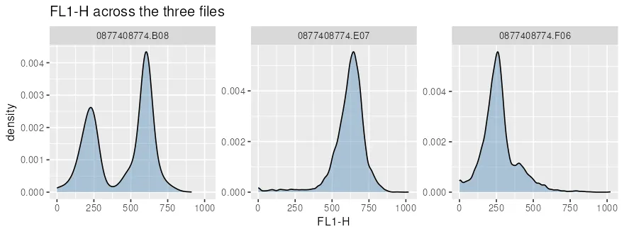

The three files do not agree. B08 is bimodal, E07 sits almost entirely in the positive range, and F06 sits almost entirely in the negative range with a small shoulder. That pattern is either three different samples, three different stains, or a problem, and the plot cannot tell you which. The sample metadata table can, which is the argument for building it before you look at anything.

ggcyto gives one panel per file without being asked, because it knows the object is a set. Three files fit on a screen and thirty do not, which is the other reason the table below stops being bookkeeping.

In a real study this table is written by hand or parsed from the file names, and it is what the gating and clustering steps receive. The rest of this section uses the bundled Bodenmiller dataset, which ships with its metadata already attached.