UMAP & Clustering

High-dimensional data is hard to cluster and impossible to eyeball. A gene-expression matrix has thousands of genes per cell; the digits used here have 64 pixels each. UMAP reduces that to two dimensions you can plot, and it keeps points that were close in the original space close in the projection. Once the natural groups are pulled apart, a plain clusterer finds them.

This page runs the whole loop on the bundled scikit-learn digits: reduce to 2D, cluster, and check the clusters against the digit labels we happen to know. Every code block runs in a container in the companion repository, so the numbers and figures are real.

Load the data

1797 handwritten digits, each an 8x8 image flattened to 64 features. Scaling matters: UMAP works on distances, so features on different scales would distort them.

from sklearn.datasets import load_digits
from sklearn.preprocessing import StandardScaler

digits = load_digits()
X = StandardScaler().fit_transform(digits.data)
y = digits.target
print(X.shape, "->", len(set(y)), "known classes (digits 0-9)")

(1797, 64) -> 10 known classes (digits 0-9)

Reduce to 2D with UMAP

Two parameters carry most of the behavior. n_neighbors sets how much local versus global structure UMAP preserves, and min_dist sets how tightly points may pack. Setting random_state makes UMAP single-threaded and deterministic, so the projection is the same on every run.

import umap

reducer = umap.UMAP(n_neighbors=15, min_dist=0.1, n_components=2, random_state=42)
embedding = reducer.fit_transform(X)
print(embedding.shape)

(1797, 2)

Cluster the projection and score it

Clustering runs on the 2D embedding rather than the raw 64 dimensions. UMAP has already separated the groups, so KMeans with ten clusters recovers them. Because the digits carry true labels, three scores say how well the clusters match: the adjusted Rand index and adjusted mutual information compare clusters to labels and are corrected for chance, and the silhouette measures how well separated the clusters are on their own.

from sklearn.cluster import KMeans
from sklearn.metrics import (adjusted_mutual_info_score, adjusted_rand_score,
                             silhouette_score)

clusters = KMeans(n_clusters=10, n_init=10, random_state=42).fit_predict(embedding)

print(f"adjusted Rand index         {adjusted_rand_score(y, clusters):.3f}")
print(f"adjusted mutual information {adjusted_mutual_info_score(y, clusters):.3f}")
print(f"silhouette (on embedding)   {silhouette_score(embedding, clusters):.3f}")

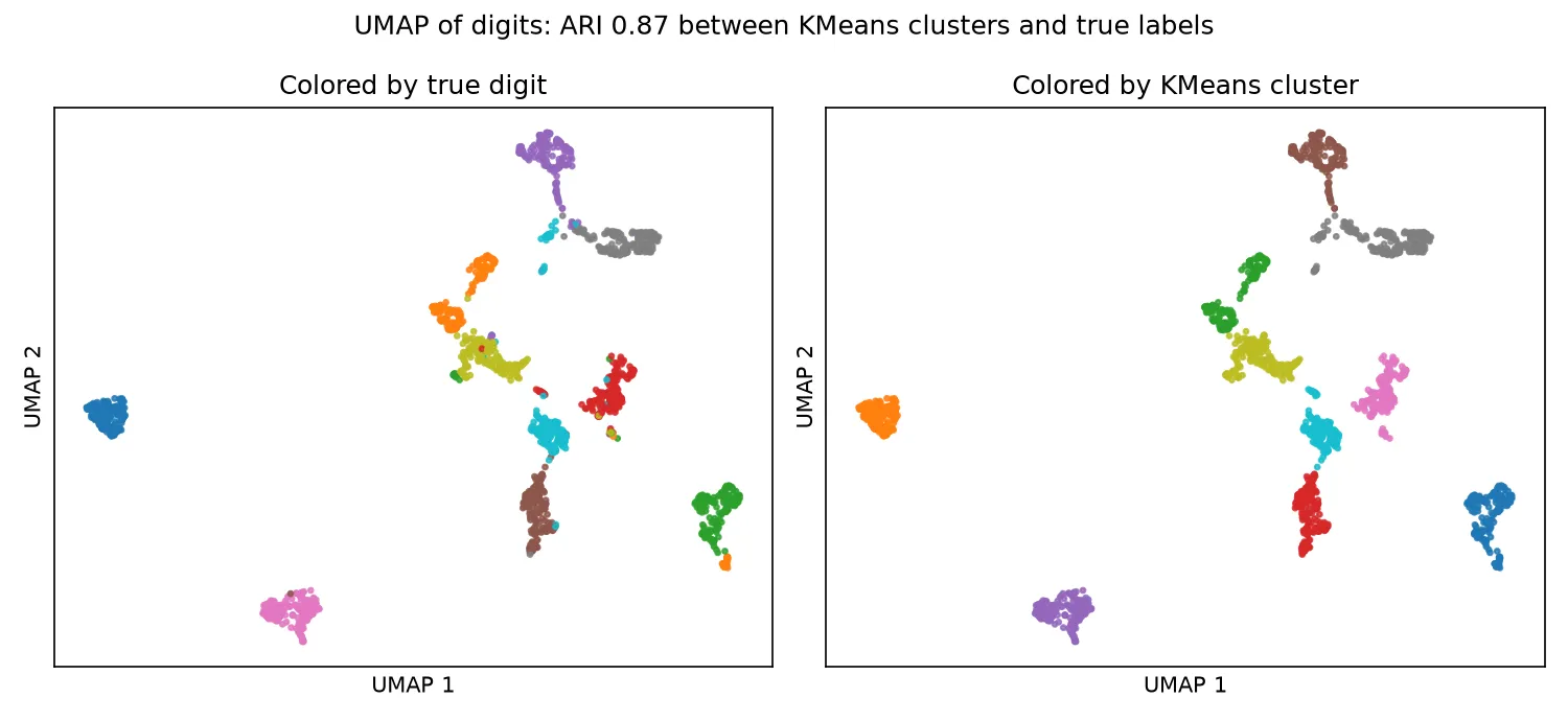
adjusted Rand index         0.871
adjusted mutual information 0.896
silhouette (on embedding)   0.705

An adjusted Rand index of 0.871 is strong. KMeans never saw the labels, yet its ten clusters line up with the ten digits almost exactly. The two panels below show why: the projection colored by true digit and by KMeans cluster are nearly the same picture. Where they disagree is the honest part, the digits that overlap in pixel space, such as 4 and 9.

The n_neighbors knob

n_neighbors is the first parameter to reach for. Small values keep the view local, so the data breaks into many tight islands. Large values pull in global structure, so you get fewer, broader groups. There is no single correct value; it depends on whether you care about fine subgroups or the overall layout. The same sweep on single-cell data is how you decide between splitting rare cell states and showing the major lineages.

for k in (5, 15, 30, 100):
    emb = umap.UMAP(n_neighbors=k, min_dist=0.1, random_state=42).fit_transform(X)
    # ... scatter emb colored by y ...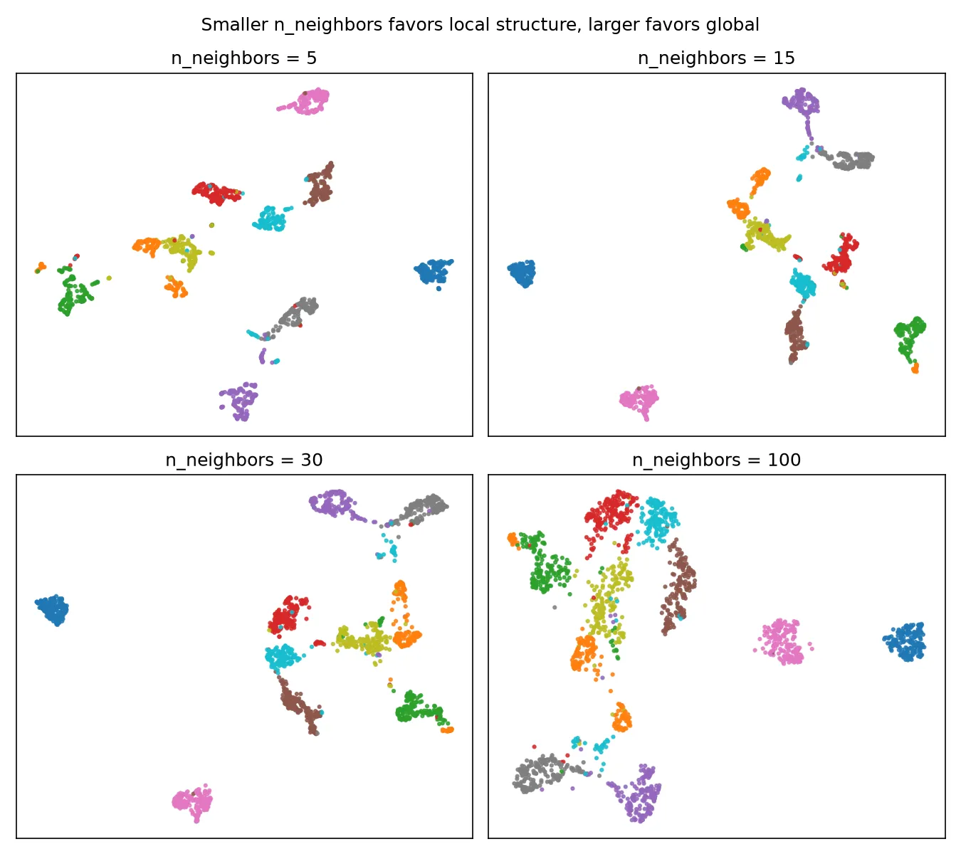

Two cautions

UMAP distances are not a metric you can read literally. The gap between two clusters in the plot does not mean they are that far apart in the original space, so do not compute distances on the embedding and treat them as real. And clustering on the embedding, while common and convenient, inherits whatever distortion UMAP introduced. When a cluster boundary matters, confirm it against the original features, not only the 2D picture.