Missing Data Mechanisms
A missing value is not a hole in a file. It is a measurement that exists and was not recorded, and what it cost you depends on why it was not recorded. Rubin’s three mechanisms classify that reason. Missing completely at random, MCAR, means the gap has nothing to do with anything else in the data. Missing at random, MAR, means the gap tracks values you did observe. Missing not at random, MNAR, means the gap tracks the value itself: the patient whose cholesterol came back extreme is the one whose lab result never reached the table.
The classification decides the analysis, and the data cannot hand it to you. MAR and MNAR are statements about values you never saw, so no test on the observed data can separate them. What the data can answer is narrower and still useful: whether missingness tracks the columns you did observe. That test is the subject of this page, and it is the difference between a complete-case analysis you can defend and one you cannot.
Every number on this page comes from a real run of the code shown, in the section’s container, in both languages.
The cohort with holes
Section titled “The cohort with holes”This section computes on one synthetic cohort of 400 patients, generated by a committed script in the companion repository: age, body mass index, activity level, smoking status, total cholesterol and systolic blood pressure. Missingness was introduced deliberately into the last four variables, and the complete version of the cohort is kept beside the missing one, so the imputation pages that follow score every method against the truth it had to reconstruct. A synthetic cohort is the honest choice here: on real data the true values behind the gaps are by definition unknown, and no evaluation number could be computed.
suppressPackageStartupMessages({  library(ggplot2)  library(mice)})
#' Format a numeric value for tutorial output.#'#' @param value A numeric value.#' @return A character string with four decimal places.FormatNumber <- function(value) {  sprintf("%.4f", value)}
cohort <- read.csv("/opt/data/cohort_missing.csv", stringsAsFactors = FALSE)cohort$activity <- factor(cohort$activity,  levels = c("low", "medium", "high"), ordered = TRUE)cohort$smoking <- factor(cohort$smoking, levels = c("0", "1"))analysis_variables <- setdiff(names(cohort), "patient_id")complete_cases <- sum(complete.cases(cohort[analysis_variables]))
cat(sprintf("Cohort dimensions: %d rows, %d columns\n",  nrow(cohort), ncol(cohort)))for (variable_name in names(cohort)) {  missing_count <- sum(is.na(cohort[[variable_name]]))  missing_percent <- 100 * missing_count / nrow(cohort)  cat(sprintf("%s: %d of %d missing (%s percent)\n", variable_name,    missing_count, nrow(cohort), sprintf("%.1f", missing_percent)  ))}cat(sprintf("Complete cases: %d\n", complete_cases))
Cohort dimensions: 400 rows, 7 columnspatient_id: 0 of 400 missing (0.0 percent)age: 0 of 400 missing (0.0 percent)bmi: 0 of 400 missing (0.0 percent)activity: 48 of 400 missing (12.0 percent)smoking: 48 of 400 missing (12.0 percent)chol: 62 of 400 missing (15.5 percent)sbp: 52 of 400 missing (13.0 percent)Complete cases: 238import pandas as pd
def format_number(value): """Format a numeric value for tutorial output.
Args: value: Numeric value to format.
Returns: A string with four decimal places. """ return f"{value:.4f}"
cohort = pd.read_csv("/opt/data/cohort_missing.csv")analysis_variables = ["age", "bmi", "activity", "smoking", "chol", "sbp"]complete_cases = int(cohort[analysis_variables].notna().all(axis=1).sum())
print(f"Cohort dimensions: {cohort.shape[0]} rows, {cohort.shape[1]} columns")for variable_name in cohort.columns: missing_count = int(cohort[variable_name].isna().sum()) missing_percent = 100 * missing_count / len(cohort) print( f"{variable_name}: {missing_count} of {len(cohort)} missing " f"({missing_percent:.1f} percent)" )print(f"Complete cases: {complete_cases}")Cohort dimensions: 400 rows, 7 columnspatient_id: 0 of 400 missing (0.0 percent)age: 0 of 400 missing (0.0 percent)bmi: 0 of 400 missing (0.0 percent)activity: 48 of 400 missing (12.0 percent)smoking: 48 of 400 missing (12.0 percent)chol: 62 of 400 missing (15.5 percent)sbp: 52 of 400 missing (13.0 percent)Complete cases: 238Both engines read the same committed CSV, and the counts agree row for row. The variables age and bmi are complete; the other four carry the gaps. Cholesterol is missing for 62 patients, blood pressure for 52, and activity and smoking for 48 each. A complete-case analysis would keep 238 of the 400 patients and discard the rest before any modelling started.
Patterns of missingness
Section titled “Patterns of missingness”The per-variable counts hide where the holes are. If every missing cell sat on a different patient, 210 missing cells would spread across 210 patients and a complete-case analysis would keep only half the cohort. If they cluster, the same count leaves far more usable rows. The pattern table shows the combinations: one row per pattern of observed and missing variables, with the number of patients who show it.
x <- cohort[analysis_variables]cat("Cohort missingness pattern table:\n")print(suppressWarnings(mice::md.pattern(x, plot = FALSE)))data(nhanes2, package = "mice")cat("nhanes2 missingness pattern table:\n")print(suppressWarnings(mice::md.pattern(nhanes2, plot = FALSE)))dir.create("outputs", showWarnings = FALSE)write.csv(nhanes2, "outputs/nhanes2.csv", row.names = FALSE)Cohort missingness pattern table: age bmi activity smoking sbp chol238 1 1 1 1 1 1 062 1 1 1 1 1 0 152 1 1 1 1 0 1 148 1 1 0 0 1 1 2 0 0 48 48 52 62 210nhanes2 missingness pattern table: age hyp bmi chl13 1 1 1 1 03 1 1 1 0 11 1 1 0 1 11 1 0 0 1 27 1 0 0 0 3 0 8 9 10 27def missing_pattern_table(frame, variables): """Count missingness patterns for the selected variables.
Args: frame: Data frame that contains the variables. variables: Variables that define a missingness pattern.
Returns: A table with each binary missingness pattern and its row count. """ pattern_series = frame[variables].isna().astype(int).astype(str).agg( "".join, axis=1 ) return pattern_series.value_counts().rename_axis( "missing_pattern" ).reset_index(name="rows")
def print_pattern_table(label, frame, variables): """Print a labelled missingness pattern table.
Args: label: Text that identifies the data frame. frame: Data frame that contains the variables. variables: Variables that define a missingness pattern.
Returns: None. """ print(f"{label} missingness pattern table:") print(missing_pattern_table(frame, variables).to_string(index=False))
print_pattern_table("Cohort", cohort, analysis_variables)nhanes2 = pd.read_csv("outputs/nhanes2.csv")print_pattern_table("nhanes2", nhanes2, list(nhanes2.columns))Cohort missingness pattern table:missing_pattern rows 000000 238 000010 62 000001 52 001100 48nhanes2 missingness pattern table:missing_pattern rows 0000 13 0111 7 0001 3 0100 1 0110 1The cohort has four patterns. Besides the 238 complete patients, 62 are missing
only cholesterol, 52 are missing only blood pressure, and 48 are missing activity
and smoking together, a co-occurrence the pattern table makes visible and the
per-variable counts could not. The second table is nhanes2, the 25-patient
teaching set that ships with mice, here so the same two displays can be compared
on data you will meet in every mice vignette. It has 13 complete patients and 27
missing cells, and its patterns nearly nest into one another, which is what the
literature calls a monotone pattern. The cohort’s patterns do not nest, and that
matters later: scattered patterns are exactly the case where iterated imputation
earns its keep.
The Python table reads a CSV that the R block wrote, because nhanes2 lives in
an R package. A zero marks an observed value in the Python encoding and a one
marks a gap, so the row 0000 with 13 patients is the same complete pattern the
R table shows first.
What the data can tell you
Section titled “What the data can tell you”You cannot test whether missingness depends on the missing values. You can test whether it depends on the observed ones. If patients with a missing cholesterol value are systematically older, then cholesterol is not MCAR, and an analysis that keeps only complete cases will compare a younger subset to the cohort you meant to study.
chol_missing <- is.na(cohort$chol)welch_test <- t.test(age ~ is.na(chol), data = cohort)age_observed_mean <- mean(cohort$age[!chol_missing])age_missing_mean <- mean(cohort$age[chol_missing])cat(sprintf("Age mean when chol observed: %s\n", FormatNumber(age_observed_mean)))cat(sprintf("Age mean when chol missing: %s\n", FormatNumber(age_missing_mean)))cat(sprintf("Welch t-test age by chol missing p-value: %.3e\n", welch_test$p.value))logit_fit <- glm(chol_missing ~ age + bmi, data = cohort, family = binomial)cat("Logit coefficient table:\n")print(coef(summary(logit_fit)))cat(sprintf("Odds ratio per year of age: %s\n", FormatNumber(exp(coef(logit_fit)["age"]))))Age mean when chol observed: 53.5355Age mean when chol missing: 62.0484Welch t-test age by chol missing p-value: 3.420e-07Logit coefficient table: Estimate Std. Error z value Pr(>|z|)(Intercept) -5.264515234 1.08404889 -4.856345 1.195724e-06age 0.062021351 0.01330418 4.661794 3.134646e-06bmi -0.000942711 0.03795744 -0.024836 9.801858e-01Odds ratio per year of age: 1.0640import numpy as npimport statsmodels.api as smfrom scipy import stats
chol_missing = cohort["chol"].isna()age_missing = cohort.loc[chol_missing, "age"]age_observed = cohort.loc[~chol_missing, "age"]welch_test = stats.ttest_ind(age_missing, age_observed, equal_var=False)print(f"Age mean when chol observed: {format_number(age_observed.mean())}")print(f"Age mean when chol missing: {format_number(age_missing.mean())}")print( "Welch t-test age by chol missing p-value: " f"{welch_test.pvalue:.3e}")x = sm.add_constant(cohort[["age", "bmi"]])logit_fit = sm.Logit(chol_missing.astype(int), x).fit(disp=False)print("Logit coefficient table:")print(logit_fit.summary2().tables[1])print( "Odds ratio per year of age: " f"{format_number(np.exp(logit_fit.params['age']))}")Age mean when chol observed: 53.5355Age mean when chol missing: 62.0484Welch t-test age by chol missing p-value: 3.420e-07Logit coefficient table: Coef. Std.Err. z P>|z| [0.025 0.975]const -5.264515 1.084049 -4.856342 0.000001 -7.389213 -3.139817age 0.062021 0.013304 4.661791 0.000003 0.035946 0.088097bmi -0.000943 0.037957 -0.024836 0.980186 -0.075338 0.073453Odds ratio per year of age: 1.0640The answer is not subtle. Patients with a missing cholesterol value average 62.0 years against 53.5 for the rest, and the logistic fit puts the odds of a missing value up by a factor of 1.064 for each additional year of age. Body mass index carries no such signal, with a coefficient of -0.0009 and a p-value of 0.98. Cholesterol missingness is therefore not MCAR; it tracks an observed variable, which is the MAR side of the fence. The two engines agree on every number here, and the companion repository’s gate checks that agreement mechanically on each run.
One caution before you build on this. The same test can never rule MNAR in or out. If the laboratory loses the extreme results more often, that dependence leaves no trace in the observed columns, and the honest position is to state the MAR assumption and return to it in a sensitivity analysis, which is what the last page of this section does.
A map of the holes
Section titled “A map of the holes”The pattern table counts; a map shows. Both figures draw the same 400 by 4 grid of cells, one tile per patient per incomplete variable, red where the value is missing. Patients are sorted so the complete cases come first, then grouped by pattern, which turns the table you just read into bands you can see.
map_variables <- c("chol", "sbp", "activity", "smoking")map_missing <- is.na(cohort[map_variables])map_pattern <- apply(map_missing, 1, paste0, collapse = "")map_complete <- complete.cases(x)map_order <- order(-as.integer(map_complete), map_pattern, cohort$patient_id)map_frame <- data.frame( variable = rep(map_variables, times = nrow(cohort)), patient = rep(seq_len(nrow(cohort)), each = length(map_variables)), missing = as.vector(t(map_missing[map_order, , drop = FALSE])))map_plot <- ggplot(map_frame, aes(x = variable, y = patient, fill = missing)) + geom_tile() + scale_fill_manual(values = c("FALSE" = "grey95", "TRUE" = "#b2182b")) + guides(fill = "none") + scale_y_reverse() + labs(x = NULL, y = "Patient order") + theme_minimal()ggsave("outputs/mechanisms_missingness_map_r.png", map_plot, width = 7, height = 4, dpi = 150)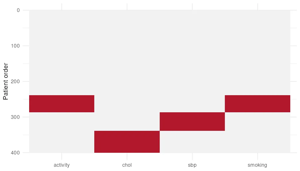
import os
import matplotlib.pyplot as pltimport numpy as np
def make_missingness_map(frame, variables, path):    """Save a map that puts complete cases before incomplete cases.
    Args:        frame: Cohort data frame.        variables: Variables that appear in the map.        path: Image output path.
    Returns:        None.    """    sorted_frame = frame.copy()    sorted_frame["missing_pattern"] = sorted_frame[        analysis_variables    ].isna().astype(int).astype(str).agg("".join, axis=1)    complete_values = sorted_frame[analysis_variables].notna()    sorted_frame["complete_case"] = complete_values.all(axis=1)    sorted_frame = sorted_frame.sort_values(        ["complete_case", "missing_pattern", "patient_id"],        ascending=[False, True, True],        kind="stable",    )    missing_matrix = sorted_frame[variables].isna().to_numpy(dtype=int)    figure, axis = plt.subplots(figsize=(7, 4))    axis.imshow(        missing_matrix,        aspect="auto",        cmap="Reds",        interpolation="none",    )    axis.set_xticks(np.arange(len(variables)), variables)    axis.set_ylabel("Patient order")    axis.set_yticks([])    figure.tight_layout()    figure.savefig(path, dpi=150)    plt.close(figure)
os.makedirs("outputs", exist_ok=True)map_variables = ["chol", "sbp", "activity", "smoking"]make_missingness_map(cohort, map_variables,                     "outputs/mechanisms_missingness_map_python.png")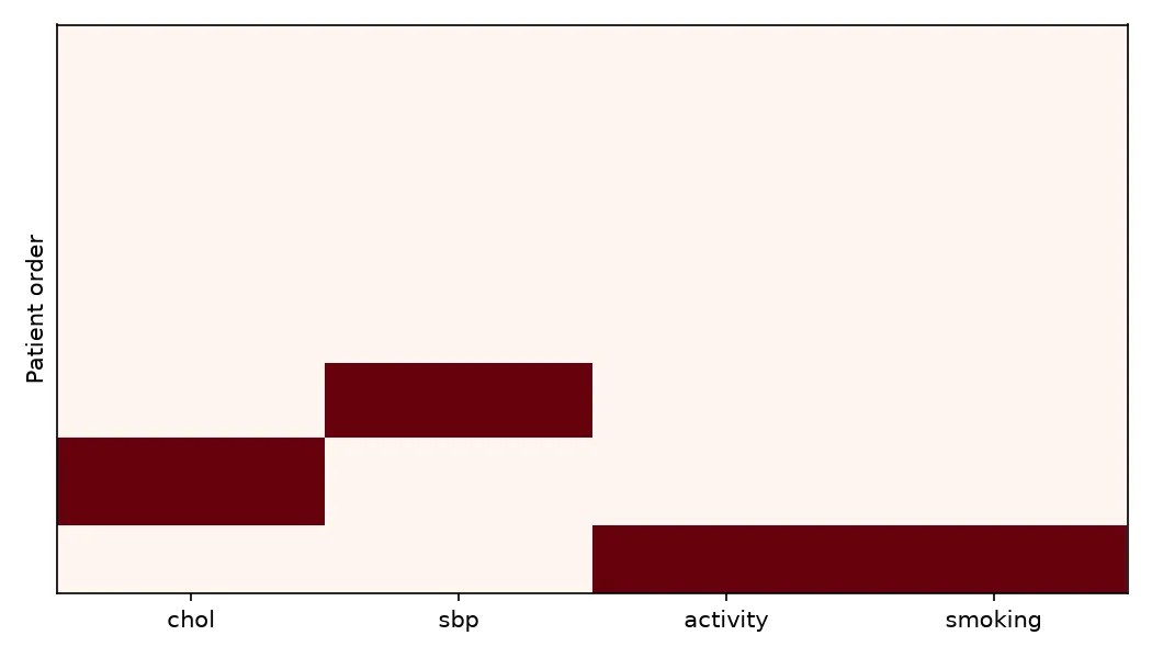
The working assumption
Section titled “The working assumption”The evidence on this page says the cohort is not MCAR, because cholesterol missingness tracks age at an odds ratio of 1.064 per year. It does not say the data is safe, because no observed-column test can see an MNAR dependence. The rest of the section works under MAR: imputation models lean on the observed columns, and the evaluation page prices what happens when that assumption is wrong by a measured amount.