Kaplan-Meier & Log-rank
Survival analysis studies the time until an event: death, relapse, or any milestone. Its defining feature is censoring. Some patients are still event-free when the study ends, so you know they survived at least that long, but not their full time. The Kaplan-Meier estimator handles this honestly. This page compares survival between two arms, in R and Python.
Every code block on this page runs in a container in the companion repository. The numbers and figure come from those real runs.
When to use Kaplan-Meier
Section titled “When to use Kaplan-Meier”Use it whenever the outcome is time-to-event with censoring. It estimates the survival curve without assuming a distribution, and the log-rank test compares curves between groups. It is the standard first look in any clinical trial with a survival endpoint.
The data
Section titled “The data”survival.csv has 120 patients in two arms. Each row has a time in months, an
event flag (1 for the event, 0 for censored), and a group.
library(survival)
df <- read.csv("survival.csv")fit <- survfit(Surv(time, event) ~ group, data = df)fit
n events median 0.95LCL 0.95UCLgroup=control 60 58 5.38 3.77 9.69group=treated 60 52 10.97 7.58 17.33import pandas as pdfrom lifelines import KaplanMeierFitter
df = pd.read_csv("survival.csv")kmf = KaplanMeierFitter()for grp in ["control", "treated"]: m = df["group"] == grp kmf.fit(df.loc[m, "time"], df.loc[m, "event"], label=grp) print(grp, kmf.median_survival_time_)control median survival: 5.47treated median survival: 11.26Median survival is about 5.4 months in the control arm and about 11 months in the treated arm. The small difference in the median between the two tools comes from how each reads the median off the step curve; the curves themselves are the same.
The survival curves
Section titled “The survival curves”The Kaplan-Meier curve is a staircase. It steps down at each event and flattens where data is only censored. The shaded band is the confidence interval.
library(survminer)
ggsurvplot(fit, data = df, conf.int = TRUE, pval = TRUE)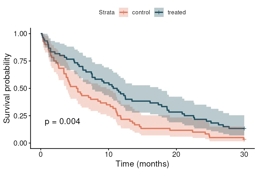
kmf.plot_survival_function()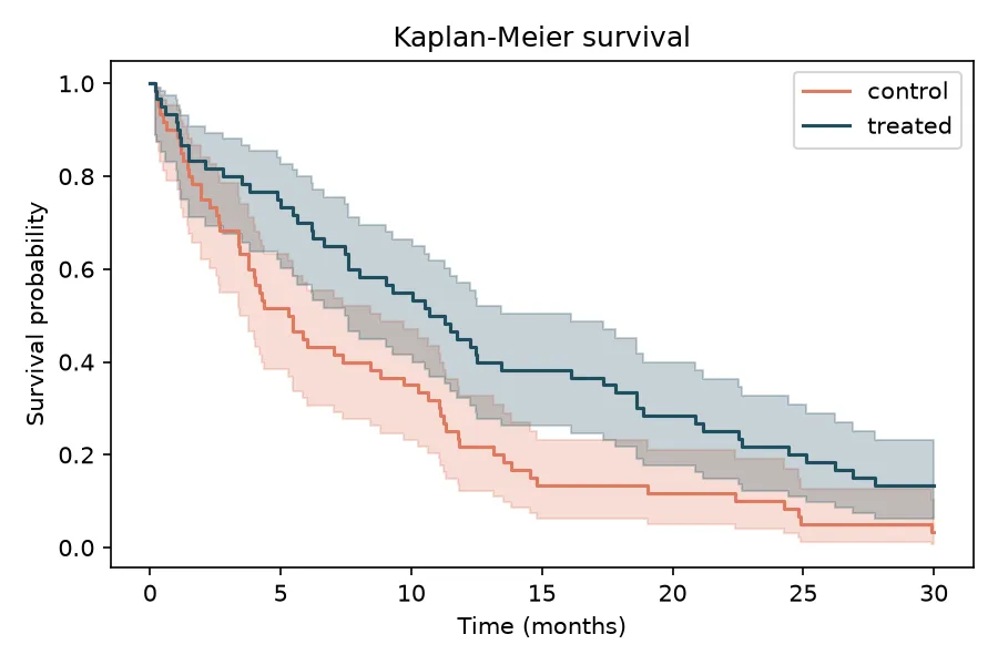
The log-rank test
Section titled “The log-rank test”Do the two curves differ by more than chance? The log-rank test compares the whole curves, weighting every event time, not just the medians.
survdiff(Surv(time, event) ~ group, data = df) N Observed Expected (O-E)^2/E (O-E)^2/Vgroup=control 60 58 43.4 4.89 8.3group=treated 60 52 66.6 3.19 8.3
Chisq= 8.3 on 1 degrees of freedom, p= 0.004from lifelines.statistics import logrank_test
c = df[df["group"] == "control"]t = df[df["group"] == "treated"]logrank_test(c["time"], t["time"], c["event"], t["event"])log-rank: chi2 = 8.304, p = 3.956e-03Both give a chi-square of 8.3 and p = 0.004. The treated arm survives significantly longer.
Pitfalls and bioinformatics notes
Section titled “Pitfalls and bioinformatics notes”- Censoring must be non-informative. The method assumes censored patients would have had the same risk as those still followed. Patients who drop out because they are sicker break that assumption.
- The median may not be reached. If more than half the arm is still event-free at the end, the median survival is undefined. Report a landmark survival, such as survival at 12 months, instead.
- The log-rank test has a blind spot. It is weak when curves cross. If the curves cross, the overall test can miss a real, time-varying difference.
- Do not dichotomize a biomarker to plot curves. Splitting a continuous marker at the median to draw two curves throws away information and inflates false positives. Model it continuously with Cox regression instead.
Key points
Section titled “Key points”- Kaplan-Meier estimates a survival curve while respecting censored observations.
- The log-rank test compares survival curves across groups over the whole follow-up.
- Report median survival, or a landmark survival when the median is not reached.
- R and Python give the same log-rank result.
Further reading
Section titled “Further reading”- STHDA, survival analysis basics.
- An Introduction to Statistical Learning, chapter 11.
- The next guide, Cox proportional hazards, which models survival with covariates.