Evaluating Imputation Quality
An imputation you have not checked is a hope, and the previous pages produced one: 20 completed cohorts and a pooled answer. This page checks it. Three of the four checks are the ones you can do on any real data set: whether the chains settled, whether the imputed values look like the observed ones, and how much the answer moves if the MAR assumption is wrong. The fourth is a luxury of this section’s fixture, where the true values behind the gaps exist and every claim can be scored against them.
Did the chains settle
Section titled “Did the chains settle”mice iterates: each incomplete variable is imputed from the others in turn, and five iterations of that loop make one chain. The trace plot draws the mean of the imputed values per iteration for each of the 20 chains. What you want to see is boring: level noise with no trend and no chain drifting apart from the others.
suppressPackageStartupMessages({  library(ggplot2)  library(mice)})
dir.create("outputs", showWarnings = FALSE, recursive = TRUE)
complete_data <- read.csv("/opt/data/cohort_complete.csv", check.names = FALSE)missing_data <- read.csv("/opt/data/cohort_missing.csv", check.names = FALSE)mask_data <- read.csv("/opt/data/amputation_mask.csv", check.names = FALSE)
factor_levels <- c("low", "medium", "high")complete_data$activity <- ordered(  complete_data$activity,  levels = factor_levels)missing_data$activity <- ordered(  missing_data$activity,  levels = factor_levels)complete_data$smoking <- factor(complete_data$smoking, levels = c(0, 1))missing_data$smoking <- factor(missing_data$smoking, levels = c(0, 1))
predictor_matrix <- make.predictorMatrix(missing_data)predictor_matrix[, "patient_id"] <- 0imp <- mice(  missing_data,  m = 20,  maxit = 5,  seed = 20260820,  predictorMatrix = predictor_matrix,  printFlag = FALSE)
trace_rows <- vector("list", length = 2 * 20 * 5)trace_index <- 1for (variable in c("chol", "sbp")) {  for (chain in seq_len(20)) {    for (iteration in seq_len(5)) {      trace_rows[[trace_index]] <- data.frame(        variable = variable,        chain = chain,        iteration = iteration,        chain_mean = imp$chainMean[variable, iteration, chain]      )      trace_index <- trace_index + 1    }  }}trace_data <- do.call(rbind, trace_rows)
# A healthy chain shows level noise with no trend across iterations.trace_plot <- ggplot(  trace_data,  aes(x = iteration, y = chain_mean, group = chain, colour = factor(chain))) +  geom_line(alpha = 0.7, show.legend = FALSE) +  facet_wrap(~ variable, scales = "free_y") +  labs(x = "Iteration", y = "Mean of imputed values") +  theme_minimal()ggsave(  "outputs/evaluating_trace_r.png",  plot = trace_plot,  width = 7,  height = 4,  dpi = 150)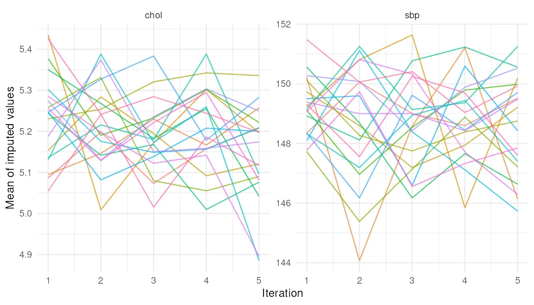
from pathlib import Pathfrom statistics import NormalDist
import matplotlib.pyplot as pltimport miceforest as mfimport numpy as npimport pandas as pdimport seaborn as snsimport statsmodels.api as sm
DATA_DIRECTORY = Path("/opt/data")OUTPUT_DIRECTORY = Path("outputs")IMPUTATIONS = 20ITERATIONS = 5SEED = 20260820MODEL_COLUMNS = ["age", "bmi", "chol", "smoking"]
def pool_rubins(fits):    """Pool OLS coefficients with Rubin's total variance.
    Args:        fits: A sequence of fitted statsmodels OLS result objects.
    Returns:        A data frame with pooled estimates, standard errors, and normal        intervals.    """    parameter_names = fits[0].params.index    estimates = np.vstack([        fit.params.loc[parameter_names].to_numpy() for fit in fits    ])    within_variances = np.vstack([        fit.bse.loc[parameter_names].to_numpy() ** 2 for fit in fits    ])    imputation_count = len(fits)    pooled_estimates = estimates.mean(axis=0)    within_variance = within_variances.mean(axis=0)    between_variance = estimates.var(axis=0, ddof=1)    total_variance = within_variance + (        1 + 1 / imputation_count    ) * between_variance    standard_errors = np.sqrt(total_variance)    critical_value = NormalDist().inv_cdf(0.975)    return pd.DataFrame({        "term": parameter_names,        "pooled_estimate": pooled_estimates,        "pooled_se": standard_errors,        "lower_2.5": pooled_estimates - critical_value * standard_errors,        "upper_97.5": pooled_estimates + critical_value * standard_errors,    })
def fit_analysis_model(data):    """Fit the tutorial analysis model to one completed data set.
    Args:        data: A completed cohort data frame.
    Returns:        A fitted statsmodels OLS result object.    """    predictors = data.loc[:, MODEL_COLUMNS].astype(float)    design_matrix = sm.add_constant(predictors, has_constant="add")    outcome = data["sbp"].astype(float)    return sm.OLS(outcome, design_matrix).fit()
def create_completed_long(kernel, patient_ids):    """Return all final completed data sets in one data frame.
    Args:        kernel: A fitted miceforest imputation kernel.        patient_ids: Patient identifiers in the imputation input row order.
    Returns:        A data frame with one dataset identifier for each completed data set.    """    completed_sets = []    for dataset_index in range(IMPUTATIONS):        completed_data = kernel.complete_data(dataset=dataset_index).copy()        completed_data.insert(0, "patient_id", patient_ids.to_numpy())        completed_data["dataset"] = dataset_index + 1        completed_sets.append(completed_data)    return pd.concat(completed_sets, ignore_index=True)
OUTPUT_DIRECTORY.mkdir(exist_ok=True)complete_data = pd.read_csv(DATA_DIRECTORY / "cohort_complete.csv")missing_data = pd.read_csv(DATA_DIRECTORY / "cohort_missing.csv")mask_data = pd.read_csv(DATA_DIRECTORY / "amputation_mask.csv")mask_columns = ["activity", "smoking", "chol", "sbp"]for column in mask_columns:    mask_data[column] = mask_data[column].astype(bool)
activity_codes = {"low": 1, "medium": 2, "high": 3}missing_for_imputation = missing_data.drop(columns="patient_id").copy()missing_for_imputation["activity"] = missing_for_imputation[    "activity"].map(activity_codes)kernel = mf.ImputationKernel(    missing_for_imputation,    num_datasets=IMPUTATIONS,    random_state=SEED,    mean_match_candidates=5,)kernel.mice(iterations=ITERATIONS, verbose=False, num_threads=1)
trace_figure, trace_axis = plt.subplots(figsize=(7, 4))imputed_chol_mask = mask_data["chol"].to_numpy()for dataset_index in range(IMPUTATIONS):    chain_means = []    for iteration in range(1, ITERATIONS + 1):        iteration_data = kernel.complete_data(            dataset=dataset_index,            iteration=iteration,        )        chain_means.append(            iteration_data.loc[imputed_chol_mask, "chol"].mean()        )    trace_axis.plot(range(1, ITERATIONS + 1), chain_means, alpha=0.7)# A healthy chain shows level noise with no trend across iterations.trace_axis.set(xlabel="Iteration", ylabel="Mean of imputed cholesterol")trace_figure.tight_layout()trace_figure.savefig(    OUTPUT_DIRECTORY / "evaluating_trace_python.png",    dpi=150,)plt.close(trace_figure)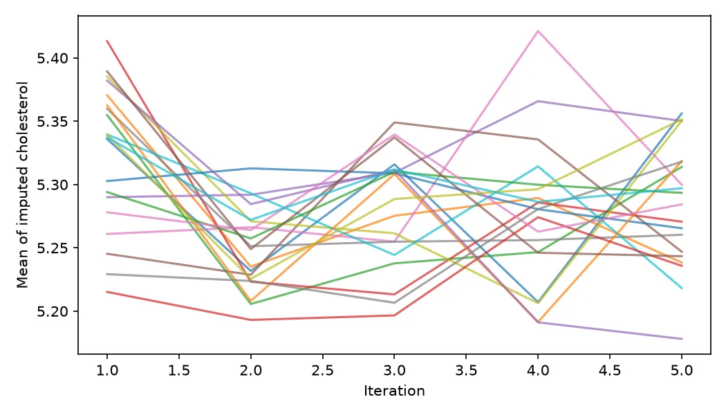
Five iterations are the mice default, and the traces show why that default is enough on this cohort: the chains reach their shared level immediately and stay there. A trend across iterations would mean the chain had not found its level yet, and the remedy would be more iterations, not more data sets.
Do the imputed values look like real ones
Section titled “Do the imputed values look like real ones”The second check draws the imputed values against the observed ones. Under MCAR the two densities should coincide. Under MAR they should not: the missing cholesterol belongs to older patients, so the imputed distribution should sit to the right of the observed one. The check is not “are they identical” but “does the difference match the mechanism”.
long_data <- complete(imp, action = "long", include = FALSE)mask_lookup <- mask_data[match(long_data$patient_id, mask_data$patient_id), ]long_data$chol_missing <- mask_lookup$chol
density_data <- rbind(  data.frame(    group = "Observed",    chol = missing_data$chol[!mask_data$chol]  ),  data.frame(    group = "Imputed",    chol = long_data$chol[long_data$chol_missing]  ))density_plot <- ggplot(  density_data,  aes(x = chol, colour = group, fill = group)) +  geom_density(alpha = 0.25) +  labs(x = "Cholesterol", y = "Density", colour = NULL, fill = NULL) +  theme_minimal()ggsave(  "outputs/evaluating_density_r.png",  plot = density_plot,  width = 7,  height = 4,  dpi = 150)
observed_chol <- missing_data$chol[!mask_data$chol]imputed_chol <- long_data$chol[long_data$chol_missing]cat(sprintf("Observed chol mean: %.4f\n", mean(observed_chol)))cat(sprintf("Observed chol SD: %.4f\n", sd(observed_chol)))cat(sprintf("Imputed chol mean: %.4f\n", mean(imputed_chol)))cat(sprintf("Imputed chol SD: %.4f\n", sd(imputed_chol)))
Observed chol mean: 4.8782Observed chol SD: 0.8597Imputed chol mean: 5.1468Imputed chol SD: 0.8625long_data = create_completed_long(kernel, missing_data["patient_id"])renamed_mask = mask_data.rename( columns={column: f"{column}_missing" for column in mask_columns})scored_data = long_data.merge( complete_data, on="patient_id", suffixes=("", "_true"),)scored_data = scored_data.merge( renamed_mask, on="patient_id", validate="many_to_one",)observed_chol = missing_data.loc[~mask_data["chol"], "chol"]imputed_chol = scored_data.loc[scored_data["chol_missing"], "chol"]
density_figure, density_axis = plt.subplots(figsize=(7, 4))sns.kdeplot(observed_chol, ax=density_axis, label="Observed", fill=True)sns.kdeplot(imputed_chol, ax=density_axis, label="Imputed", fill=True)density_axis.set(xlabel="Cholesterol", ylabel="Density")density_axis.legend()density_figure.tight_layout()density_figure.savefig( OUTPUT_DIRECTORY / "evaluating_density_python.png", dpi=150,)plt.close(density_figure)
print(f"Observed chol mean: {observed_chol.mean():.4f}")print(f"Observed chol SD: {observed_chol.std(ddof=1):.4f}")print(f"Imputed chol mean: {imputed_chol.mean():.4f}")print(f"Imputed chol SD: {imputed_chol.std(ddof=1):.4f}")Observed chol mean: 4.8782Observed chol SD: 0.8597Imputed chol mean: 5.2845Imputed chol SD: 0.8227Both engines shift the imputed distribution to the right, 5.1468 in R and 5.2845 in Python against an observed mean of 4.8782, and both keep its shape: the imputed standard deviation is 0.8625 in R and 0.8227 in Python against 0.8597 observed. The shift is the mechanism from the first page doing its work. The mechanisms page measured that cholesterol goes missing on older patients; older patients carry higher cholesterol; the imputation puts that cholesterol back.
Scored against the truth
Section titled “Scored against the truth”The fixture keeps the true values, so this page can compute what no real analysis can: the per-cell error of every imputed value.
mask_lookup <- mask_data[match(long_data$patient_id, mask_data$patient_id), ]long_data$sbp_missing <- mask_lookup$sbplong_data$activity_missing <- mask_lookup$activitylong_data$smoking_missing <- mask_lookup$smoking
truth_data <- complete_data[, c(  "patient_id", "activity", "smoking", "chol", "sbp")]names(truth_data)[-1] <- paste0(names(truth_data)[-1], "_true")mask_for_join <- mask_data[, c(  "patient_id", "activity", "smoking", "chol", "sbp")]names(mask_for_join)[-1] <- paste0(names(mask_for_join)[-1], "_missing")missing_columns <- names(mask_for_join)[-1]scoring_data <- long_data[, !names(long_data) %in% missing_columns]scored_data <- merge(scoring_data, truth_data, by = "patient_id", sort = FALSE)scored_data <- merge(  scored_data,  mask_for_join,  by = "patient_id",  sort = FALSE)
chol_errors <- scored_data$chol[scored_data$chol_missing] -  scored_data$chol_true[scored_data$chol_missing]sbp_errors <- scored_data$sbp[scored_data$sbp_missing] -  scored_data$sbp_true[scored_data$sbp_missing]activity_match <- scored_data$activity[scored_data$activity_missing] ==  scored_data$activity_true[scored_data$activity_missing]smoking_match <- scored_data$smoking[scored_data$smoking_missing] ==  scored_data$smoking_true[scored_data$smoking_missing]mean_chol <- mean(missing_data$chol, na.rm = TRUE)baseline_errors <- mean_chol - complete_data$chol[mask_data$chol]
cat(sprintf("chol bias: %.4f\n", mean(chol_errors)))cat(sprintf("chol RMSE: %.4f\n", sqrt(mean(chol_errors ^ 2))))cat(sprintf("sbp bias: %.4f\n", mean(sbp_errors)))cat(sprintf("sbp RMSE: %.4f\n", sqrt(mean(sbp_errors ^ 2))))cat(sprintf("activity accuracy: %.1f%%\n", 100 * mean(activity_match)))cat(sprintf("smoking accuracy: %.1f%%\n", 100 * mean(smoking_match)))cat(sprintf(  "Mean-imputation chol RMSE: %.4f\n",  sqrt(mean(baseline_errors ^ 2))))
chol bias: -0.1874chol RMSE: 0.9635sbp bias: -0.5356sbp RMSE: 16.9025activity accuracy: 37.8%smoking accuracy: 60.4%Mean-imputation chol RMSE: 0.9530chol_scored = scored_data.loc[scored_data["chol_missing"]]sbp_scored = scored_data.loc[scored_data["sbp_missing"]]chol_errors = chol_scored["chol"] - chol_scored["chol_true"]sbp_errors = sbp_scored["sbp"] - sbp_scored["sbp_true"]activity_scored = scored_data.loc[scored_data["activity_missing"]]smoking_scored = scored_data.loc[scored_data["smoking_missing"]]activity_truth = activity_scored["activity_true"].map(activity_codes)activity_accuracy = (activity_scored["activity"] == activity_truth).mean()smoking_accuracy = ( smoking_scored["smoking"] == smoking_scored["smoking_true"]).mean()mean_chol = missing_data["chol"].mean()baseline_errors = mean_chol - complete_data.loc[mask_data["chol"], "chol"]
print(f"chol bias: {chol_errors.mean():.4f}")print(f"chol RMSE: {np.sqrt(np.mean(chol_errors ** 2)):.4f}")print(f"sbp bias: {sbp_errors.mean():.4f}")print(f"sbp RMSE: {np.sqrt(np.mean(sbp_errors ** 2)):.4f}")print(f"activity accuracy: {100 * activity_accuracy:.1f}%")print(f"smoking accuracy: {100 * smoking_accuracy:.1f}%")print( f"Mean-imputation chol RMSE: {np.sqrt(np.mean(baseline_errors ** 2)):.4f}")chol bias: -0.0497chol RMSE: 0.8151sbp bias: -1.9077sbp RMSE: 14.5763activity accuracy: 45.8%smoking accuracy: 75.3%Mean-imputation chol RMSE: 0.9530Read the R numbers first, because they carry the lesson. The cholesterol RMSE under mice is 0.9635, and plain mean imputation scored 0.9530: the sophisticated engine lost to the page-2 straw man on per-cell error. That is not a malfunction. Per-cell RMSE is minimised by the conditional mean, and mean imputation is the cheapest conditional mean there is; a proper imputation draws from the conditional distribution instead, which is exactly what restores the spread the mean destroyed. miceforest’s 0.8151 happens to beat both, and activity and smoking accuracy sit near their guess-the-mode baselines in both engines. Per-cell scores are the wrong scoreboard for imputation. The right one is the next table.
The check that matters: coverage
Section titled “The check that matters: coverage”The purpose of imputation is not pretty imputed values. It is that the pooled intervals contain the answer the complete data would have given.
benchmark_fit <- lm(sbp ~ age + bmi + chol + smoking, data = complete_data)pooled_fit <- pool(with(imp, lm(sbp ~ age + bmi + chol + smoking)))pooled_summary <- summary(pooled_fit, conf.int = TRUE)benchmark <- coef(benchmark_fit)coverage_table <- data.frame( term = sub("smoking1", "smoking", pooled_summary$term), benchmark_estimate = unname(benchmark[pooled_summary$term]), pooled_estimate = pooled_summary$estimate, lower_2.5 = pooled_summary[["2.5 %"]], upper_97.5 = pooled_summary[["97.5 %"]])coverage_table$covered <- with( coverage_table, benchmark_estimate >= lower_2.5 & benchmark_estimate <= upper_97.5)cat("Interval coverage of the complete-data fit:\n")print(coverage_table, row.names = FALSE)Interval coverage of the complete-data fit: term benchmark_estimate pooled_estimate lower_2.5 upper_97.5 covered (Intercept) 61.3338564 61.2131164 51.3036533 71.122579 TRUE age 0.8968146 0.9265704 0.8085546 1.044586 TRUE bmi 0.7016504 0.6917429 0.3404333 1.043053 TRUE chol 3.0369699 2.8645593 1.0365709 4.692548 TRUE smoking 8.9983663 7.9024109 5.0177961 10.787026 TRUEbenchmark_fit = fit_analysis_model(complete_data)completed_sets = [ kernel.complete_data(dataset=dataset_index) for dataset_index in range(IMPUTATIONS)]pooled_results = pool_rubins([ fit_analysis_model(completed_data) for completed_data in completed_sets])benchmark = benchmark_fit.params.rename("benchmark_estimate")coverage_table = pooled_results.merge( benchmark, left_on="term", right_index=True, validate="one_to_one",)coverage_table["covered"] = ( (coverage_table["benchmark_estimate"] >= coverage_table["lower_2.5"]) & (coverage_table["benchmark_estimate"] <= coverage_table["upper_97.5"]))coverage_table["covered"] = np.where( coverage_table["covered"], "TRUE", "FALSE",)coverage_table["term"] = coverage_table["term"].replace({ "const": "(Intercept)"})coverage_table = coverage_table.loc[:, [ "term", "benchmark_estimate", "pooled_estimate", "lower_2.5", "upper_97.5", "covered",]]print("Interval coverage of the complete-data fit:")print(coverage_table.to_string(index=False))Interval coverage of the complete-data fit: term benchmark_estimate pooled_estimate lower_2.5 upper_97.5 covered(Intercept) 61.333856 61.919108 53.293036 70.545179 TRUE age 0.896815 0.880256 0.774316 0.986195 TRUE bmi 0.701650 0.561628 0.240791 0.882465 TRUE chol 3.036970 3.785598 2.167812 5.403385 TRUE smoking 8.998366 8.508417 6.121076 10.895758 TRUEEvery term, both engines, TRUE. The pooled intervals price the fabrication honestly enough to contain the complete-data fit. One fixture and one mechanism is not a proof, but this is the property that has to hold, and it holds here for both engines.
What if MAR is wrong
Section titled “What if MAR is wrong”The mechanisms page said the data cannot test MAR against MNAR. What you can do is state the alternative precisely and price it. A delta adjustment supposes the missing cholesterol runs systematically higher or lower than the observed pattern implies, by half a mmol/L in each direction, and repools the analysis in that world.
completed_sets <- complete(imp, action = "all")# The zero line is MAR. Other lines price lower or higher missing cholesterol.for (delta in c(-0.5, 0, 0.5)) { sensitivity_fits <- vector("list", length(completed_sets)) for (dataset_index in seq_along(completed_sets)) { sensitivity_data <- completed_sets[[dataset_index]] sensitivity_data$chol[mask_data$chol] <- sensitivity_data$chol[mask_data$chol] + delta sensitivity_fits[[dataset_index]] <- lm( sbp ~ age + bmi + chol + smoking, data = sensitivity_data ) } sensitivity_summary <- summary(pool(sensitivity_fits)) chol_row <- sensitivity_summary[sensitivity_summary$term == "chol", ] cat(sprintf( "delta = %.1f: pooled chol coefficient %.4f (SE %.4f)\n", delta, chol_row$estimate, chol_row$std.error ))}delta = -0.5: pooled chol coefficient 2.9594 (SE 0.8819)delta = 0.0: pooled chol coefficient 2.8646 (SE 0.9261)delta = 0.5: pooled chol coefficient 2.4499 (SE 0.9183)# The zero line is MAR. Other lines price lower or higher missing cholesterol.for delta in (-0.5, 0, 0.5): sensitivity_fits = [] for completed_data in completed_sets: sensitivity_data = completed_data.copy() sensitivity_data.loc[imputed_chol_mask, "chol"] += delta sensitivity_fits.append(fit_analysis_model(sensitivity_data)) sensitivity_results = pool_rubins(sensitivity_fits) chol_result = sensitivity_results.loc[ sensitivity_results["term"] == "chol" ].iloc[0] print( f"delta = {delta:.1f}: pooled chol coefficient " f"{chol_result['pooled_estimate']:.4f} " f"(SE {chol_result['pooled_se']:.4f})" )delta = -0.5: pooled chol coefficient 3.9038 (SE 0.8087)delta = 0.0: pooled chol coefficient 3.7856 (SE 0.8254)delta = 0.5: pooled chol coefficient 3.2360 (SE 0.7943)The MAR answer is the middle line, 2.8646 in R and 3.7856 in Python. If the missing cholesterol is systematically half a unit higher than MAR assumes, the estimate falls to 2.4499 in R and 3.2360 in Python, still the same side of the clinical noise floor, and if it runs half a unit lower the estimate rises. The sensitivity analysis never proves MAR. It tells you the size of the lie you would be telling if MAR failed, and leaves the judgement of whether that size matters to you.
The section’s working checklist is the four blocks above: traces that settled, imputed distributions whose difference matches the mechanism, intervals that cover, and a priced alternative to the assumption. On real data the third block does not exist, and the other three carry the whole argument.