Identifying Cells from Clusters

Clustering finds populations. It does not name them. The clustering page ends with a table of marker medians and the instruction to read it and call each cluster a cell type, which is the step everyone does by eye and nobody writes down.

Writing it down is worth the effort. A table of rules, one row per cell type, is a text file a reviewer can read and a version control system can diff, in the same way a gating template is. It also makes the annotation reproducible across samples and across people.

The definitions

Each row names a cell type and gives an expectation for the markers that define it. A marker can be pos, neg, high, or blank when it does not matter for that population. This file ships beside the guide’s code, so the page prints the file the annotation reads.

library(flowCore)
library(FlowSOM)
library(HDCytoData)

definitions <- read.csv("cell_type_definitions.csv", check.names = FALSE)
definitions[, c("cell_type", "CD3", "CD4", "CD20", "CD14", "CD123", "CD7")]

             cell_type CD3 CD4 CD20 CD14 CD123 CD7
1          CD4 T cells pos pos  neg
2 CD4 negative T cells pos neg  neg            pos
3              B cells neg      pos
4            Monocytes neg      neg  pos
5      Dendritic cells neg      neg  neg  high
6             NK cells neg      neg            pos
7               Debris neg neg  neg  neg   neg neg

The panel here has no CD8, so the second T cell row is defined by the absence of CD4 rather than the presence of CD8. Saying that in the table is better than leaving a reader to wonder why the CD8 row is missing.

Clustering the whole set

The Bodenmiller BCR-XL data is sixteen samples, eight patients measured stimulated and unstimulated. Clustering all of them together means one set of clusters covers every sample, which is what you want before comparing populations between conditions.

fs <- Bodenmiller_BCR_XL_flowSet()

# Arcsinh transform the surface markers, cofactor 5, then shorten the channel
# names to the bare marker so the definitions table can name them.
cd_channels <- grep("^CD", colnames(fs), value = TRUE)
asinh_trans <- arcsinhTransform(a = 0, b = 1 / 5, c = 0)
fs <- transform(fs, transformList(cd_channels, tfun = asinh_trans))
colnames(fs) <- sub("\\(.*$", "", colnames(fs))

markers <- grep("^CD", colnames(fs), value = TRUE)
markers

set.seed(1)
fom <- FlowSOM(fs, colsToUse = markers, nClus = 12, seed = 1)

# One row per SOM node, and the metacluster each node belongs to.
node_codes <- fom$map$codes
meta <- fom$metaclustering
length(unique(meta))

[1] "CD3"   "CD45"  "CD4"   "CD20"  "CD33"  "CD123" "CD14"  "CD7"
[1] 12

Median expression per cluster

Each metacluster gets one median per marker. That table is the input to the naming step, and it is also the thing to look at when a label surprises you.

#' Median marker expression for each metacluster.
#'
#' @param codes The SOM codebook, one row per node.
#' @param clusters The metacluster label of each node.
#' @return A data frame with one row per metacluster and one column per marker.
ClusterMedians <- function(codes, clusters) {
  levels_present <- sort(unique(clusters))
  medians <- t(vapply(levels_present, function(group) {
    apply(codes[clusters == group, , drop = FALSE], 2, median)
  }, numeric(ncol(codes))))
  out <- as.data.frame(medians)
  # metaclustering is a factor, so carry the label as a character column and
  # keep every other column numeric.
  out$cluster <- as.character(levels_present)
  out
}

median_expression <- ClusterMedians(node_codes, meta)

shown <- c("CD3", "CD4", "CD20", "CD14", "CD7")
cbind(cluster = median_expression$cluster,
      round(median_expression[, shown], 2))

   cluster   CD3  CD4 CD20 CD14  CD7
1        1  3.50 3.72 0.12 0.06 3.09
2        2  3.45 3.55 0.29 0.10 0.26
3        3  1.40 2.24 0.85 0.43 0.11
4        4  0.11 0.04 0.12 0.11 3.80
5        5  1.87 0.60 0.23 1.39 0.49
6        6  2.76 0.17 0.16 0.09 0.17
7        7  3.11 0.08 0.10 0.23 3.63
8        8 -0.10 0.16 0.16 0.40 0.23
9        9  0.99 0.62 0.39 0.76 0.57
10      10  1.54 0.15 0.18 0.48 3.80
11      11 -0.03 0.19 0.08 0.18 0.31
12      12  0.23 0.25 4.23 0.36 0.28

Scoring a cluster against the rules

Every marker is scaled across clusters to run from zero to one, so a bright marker and a dim one carry the same weight. A definition then adds the scaled value where it expects pos, subtracts it where it expects neg, and counts high twice.

The score is a weighted mean and not a sum, and the reason is worth stating. Under a sum, a definition is rewarded simply for naming more markers, so the most specific row in the table wins every cluster including the obvious ones. Dividing by the total weight removes that.

#' Score each cluster against each definition and take the best match.
#'
#' @param medians The output of [ClusterMedians()].
#' @param definitions The definitions table.
#' @return A data frame with the cluster, its best cell type, the score, the
#'   runner up and the margin between them.
AnnotateClusters <- function(medians, definitions) {
  marker_columns <- intersect(
    setdiff(colnames(definitions), c("cell_type", "note")),
    colnames(medians)
  )

  #' Scale one marker across clusters to run from zero to one.
  #'
  #' @param x The marker's median in each cluster.
  #' @return The scaled values, or 0.5 everywhere when the marker is constant.
  ScaleColumn <- function(x) {
    span <- max(x) - min(x)
    if (span == 0) rep(0.5, length(x)) else (x - min(x)) / span
  }
  scaled <- as.data.frame(lapply(medians[, marker_columns], ScaleColumn))

  scores <- vapply(seq_len(nrow(definitions)), function(d) {
    total <- rep(0, nrow(scaled))
    weight <- 0
    for (marker in marker_columns) {
      expectation <- definitions[d, marker]
      if (is.na(expectation) || expectation == "") next
      contribution <- switch(
        expectation,
        pos = scaled[[marker]],
        high = 2 * scaled[[marker]],
        neg = 1 - scaled[[marker]],
        NULL
      )
      if (is.null(contribution)) next
      total <- total + contribution
      weight <- weight + if (expectation == "high") 2 else 1
    }
    if (weight == 0) rep(0, nrow(scaled)) else total / weight
  }, numeric(nrow(scaled)))
  colnames(scores) <- definitions$cell_type

  ranked <- apply(scores, 1, function(row) sort(row, decreasing = TRUE)[1:2])
  data.frame(
    cluster = medians$cluster,
    cell_type = colnames(scores)[apply(scores, 1, which.max)],
    score = round(ranked[1, ], 3),
    runner_up = round(ranked[2, ], 3),
    margin = round(ranked[1, ] - ranked[2, ], 3)
  )
}

annotation <- AnnotateClusters(median_expression, definitions)
annotation

   cluster            cell_type score runner_up margin
1        1          CD4 T cells 0.989     0.752  0.236
2        2          CD4 T cells 0.973     0.606  0.367
3        3          CD4 T cells 0.693     0.644  0.049
4        4             NK cells 0.953     0.786  0.167
5        5            Monocytes 0.876     0.685  0.191
6        6               Debris 0.764     0.746  0.019
7        7 CD4 negative T cells 0.958     0.754  0.204
8        8               Debris 0.945     0.503  0.442
9        9      Dendritic cells 0.682     0.642  0.040
10      10 CD4 negative T cells 0.859     0.854  0.005
11      11               Debris 0.849     0.728  0.121
12      12              B cells 0.923     0.658  0.265

Reading the margin

The margin is the gap between the best score and the second best. A large margin means the cluster matched one definition and nothing else came close. A small one means the label is a coin toss between two populations, and a report that does not say so is hiding the weakest part of its own analysis.

# The closest calls first.
annotation[order(annotation$margin), c("cluster", "cell_type", "margin")]

   cluster            cell_type margin
10      10 CD4 negative T cells  0.005
6        6               Debris  0.019
9        9      Dendritic cells  0.040
3        3          CD4 T cells  0.049
11      11               Debris  0.121
4        4             NK cells  0.167
5        5            Monocytes  0.191
7        7 CD4 negative T cells  0.204
1        1          CD4 T cells  0.236
12      12              B cells  0.265
2        2          CD4 T cells  0.367
8        8               Debris  0.442

The heatmap, labelled

library(ggplot2)

dir.create("outputs", showWarnings = FALSE, recursive = TRUE)

heatmap_data <- do.call(rbind, lapply(markers, function(marker) {
  values <- median_expression[[marker]]
  span <- max(values) - min(values)
  data.frame(
    marker = marker,
    cluster = median_expression$cluster,
    label = paste0(median_expression$cluster, ": ", annotation$cell_type),
    scaled = if (span == 0) 0.5 else (values - min(values)) / span
  )
}))

heatmap_plot <- ggplot(heatmap_data,
                       aes(x = marker, y = label, fill = scaled)) +
  geom_tile() +
  scale_fill_viridis_c(name = "scaled median") +
  labs(title = "Metacluster marker medians, with the assigned label",
       x = NULL, y = NULL) +
  theme_minimal() +
  theme(axis.text.x = element_text(angle = 45, hjust = 1))

ggsave("outputs/cyto-cluster-annotation.png", heatmap_plot,
       width = 8, height = 5, dpi = 110, bg = "white")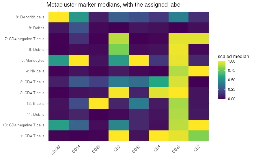

The labels the heatmap supports are the ones with a large margin. Cluster 12 is bright on CD20 and nothing else, cluster 5 carries CD14 and CD33 together, cluster 9 is the only one bright on CD123, and cluster 8 is dark everywhere, which is what debris looks like.

Cluster 6 is the one to distrust, and its margin of 0.019 says so before you look. It carries CD3 and CD7 signal, so calling it debris is wrong; what it actually is cannot be settled from these eight markers. The right move is to widen the panel or leave the cluster unnamed, not to accept the label because the script produced one.

What this does and does not give you

The table turns a clustering into named populations without anyone drawing a gate, and it records the decision in a file rather than in a person’s memory. That is the gain.

It does not tell you the definitions are right. A rule table encodes the same expert judgement a gating strategy does, and a population absent from the table cannot be found by it. What the margin column adds is an honest signal about which labels to trust, which a gating hierarchy never gives you at all.