limma-voom

limma is one of the oldest and most trusted packages in Bioconductor. It was originally designed for microarray data. The voom transformation extends limma to work with RNA-seq count data. Together they form a fast and flexible framework for differential expression analysis.

How limma-voom works

RNA-seq counts have a specific property: genes with higher expression also have higher variance. This is called the mean-variance relationship. The voom function models this relationship and assigns a precision weight to each observation. limma then uses these weights in its linear model fitting. This approach converts the count data problem into a standard linear modeling problem that limma handles well.

Loading the airway data

We use the same airway dataset from Himes et al. 2014 that we used in the DESeq2 page.

library(tidyverse)
library(airway)
library(edgeR)
library(limma)

data("airway")

counts <- assay(airway, "counts")
metadata <- colData(airway) |>
  as_tibble(rownames = "sample") |>
  select(sample, cell, dex)

# airway ships dex with trt as its first level, so model.matrix would name the
# coefficient dexuntrt and it would measure the comparison backwards. Make untrt
# the reference, which is what the DESeq2 page does too.
metadata$dex <- relevel(factor(metadata$dex), ref = "untrt")
levels(metadata$dex)

Creating a DGEList

The first step is to create a DGEList object from the edgeR package. This holds the count matrix and sample information together. limma-voom requires this format as input.

dge <- DGEList(
  counts = counts,
  samples = metadata
)

dim(dge)

[1] 63677     8

The object starts with 63,677 genes and 8 samples.

Library sizes

dge$samples$lib.size

[1] 20637971 18809481 25348649 15163415 24448408 30818215 19126151 21164133

Library sizes vary from about 15 million to 31 million reads across samples. This variation must be accounted for during normalization.

Filtering low-count genes

The filterByExpr function provides a principled way to remove genes with insufficient counts. It uses the experimental design to determine the minimum count threshold. A gene must have a sufficient number of reads in the smallest group to be retained.

keep <- filterByExpr(dge, group = metadata$dex)
dge <- dge[keep, , keep.lib.sizes = FALSE]
nrow(dge)

[1] 15926

This filter is more aggressive than our DESeq2 filter. It retains 15,926 genes compared to 22,369. The stricter filtering is appropriate because limma benefits from removing noisy low-count genes before the voom transformation.

TMM normalization

Trimmed Mean of M-values normalization corrects for composition bias. This bias arises when a few highly expressed genes consume a large fraction of the sequencing reads in some samples, leaving fewer reads for other genes. TMM calculates normalization factors that adjust for this.

dge <- calcNormFactors(dge, method = "TMM")
dge$samples$norm.factors

[1] 1.0554452 1.0212137 0.9904567 0.9484696 1.0309324 0.9779832 1.0269341
[8] 0.9538599

Normalization factors close to 1 indicate that the sample composition is similar to the reference. Values above 1 mean the sample has slightly more high-count genes. Values below 1 mean the opposite.

Design matrix

The design matrix encodes the experimental setup. We include cell line and treatment, just as we did in DESeq2.

design <- model.matrix(~ cell + dex, data = metadata)
design

  (Intercept) cellN061011 cellN080611 cellN61311 dextrt
1           1           0           0          1      0
2           1           0           0          1      1
3           1           0           0          0      0
4           1           0           0          0      1
5           1           0           1          0      0
6           1           0           1          0      1
7           1           1           0          0      0
8           1           1           0          0      1
attr(,"assign")
[1] 0 1 1 1 2
attr(,"contrasts")
attr(,"contrasts")$cell
[1] "contr.treatment"

attr(,"contrasts")$dex
[1] "contr.treatment"

Each row is a sample. The dextrt column is the coefficient of interest. It will capture the log2 fold change between treated and untreated samples after accounting for cell line differences.

voom transformation

# voom draws the mean-variance trend to the current device, so open a file
# device around it and the figure below is the one this code produced.
dir.create("outputs", showWarnings = FALSE, recursive = TRUE)
png("outputs/limma-voom-plot.png", width = 800, height = 600)
v <- voom(dge, design, plot = TRUE)
dev.off()

The voom function does three things:

Converts counts to log-counts-per-million values.
Estimates the mean-variance trend from the data.
Computes precision weights for each observation based on the trend.

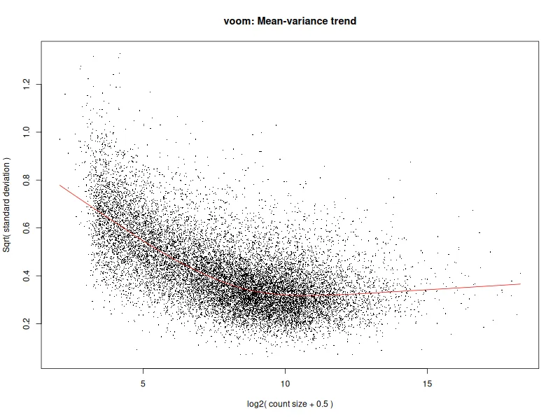
voom mean-variance plot showing the relationship between mean expression and variance

The voom plot shows the mean-variance trend. Each point is a gene. The x-axis is the average log2 count-per-million. The y-axis is the square root of the residual standard deviation. The red line is the fitted trend. Low-expression genes have higher variance. The trend flattens out for highly expressed genes. This curve is used to assign precision weights.

Fitting the linear model

limma fits the model in two steps. First, lmFit fits a linear model for each gene using the voom weights. Then, eBayes applies empirical Bayes shrinkage to the variance estimates. This borrows information across genes to improve the estimates, especially for genes with few replicates.

fit <- lmFit(v, design)
fit <- eBayes(fit)

Available coefficients

colnames(fit$coefficients)

[1] "(Intercept)" "cellN061011" "cellN080611" "cellN61311"  "dextrt"

The dextrt coefficient is our treatment effect.

Extracting results

topTable(fit, coef = "dextrt", number = 10) |>
  as_tibble(rownames = "gene")

# A tibble: 10 × 7
   gene            logFC AveExpr     t  P.Value  adj.P.Val     B
   <chr>           <dbl>   <dbl> <dbl>    <dbl>      <dbl> <dbl>
 1 ENSG00000165995  3.28    3.68  33.8 1.20e-10 0.00000192  14.3
 2 ENSG00000120129  2.94    6.65  28.4 5.57e-10 0.00000207  13.7
 3 ENSG00000157214  1.97    6.79  27.6 7.23e-10 0.00000207  13.5
 4 ENSG00000162493  1.88    5.19  27.5 7.39e-10 0.00000207  13.4
 5 ENSG00000189221  3.33    5.95  26.8 9.26e-10 0.00000207  13.2
 6 ENSG00000162614  2.03    7.64  26.1 1.17e- 9 0.00000207  13.0
 7 ENSG00000101347  3.76    8.14  25.6 1.37e- 9 0.00000207  12.8
 8 ENSG00000125148  2.20    7.02  25.6 1.39e- 9 0.00000207  12.8
 9 ENSG00000139132  2.22    5.42  25.3 1.52e- 9 0.00000207  12.7
10 ENSG00000106976 -1.77    5.10 -25.2 1.57e- 9 0.00000207  12.7

The output columns are:

logFC: The log2 fold change. Same interpretation as DESeq2.
AveExpr: The average log2 expression across all samples.
t: The moderated t-statistic from empirical Bayes.
P.Value: The raw p-value.
adj.P.Val: The Benjamini-Hochberg adjusted p-value.
B: The log-odds that the gene is differentially expressed.

The top genes overlap heavily with the DESeq2 results. ENSG00000165995, ENSG00000120129, ENSG00000101347 and ENSG00000189221 are in the top ten here and in the DESeq2 top five. The one that does not carry over is ENSG00000152583, which DESeq2 ranks first and limma-voom leaves outside its top ten, because the two rank on different statistics over different gene sets.

Significant gene counts

topTable(fit, coef = "dextrt", number = Inf) |>
  as_tibble(rownames = "gene") |>
  summarize(
    total = n(),
    sig = sum(adj.P.Val < 0.05),
    up = sum(adj.P.Val < 0.05 & logFC > 0),
    down = sum(adj.P.Val < 0.05 & logFC < 0)
  )

# A tibble: 1 × 4
  total   sig    up  down
  <int> <int> <int> <int>
1 15926  5014  2582  2432

limma-voom finds 5014 significant genes at FDR < 0.05, against 4000 from DESeq2 on the same samples. It calls more genes while testing fewer of them, 15926 against 22369, so the difference is not the filter alone. The empirical Bayes variance shrinkage that limma applies gives it more power on a design this small.

Visualizing the results

Volcano plot

library(ggplot2)

volcano_data <- topTable(fit, coef = "dextrt", number = Inf) |>
  as_tibble(rownames = "gene") |>
  mutate(significant = adj.P.Val < 0.05 & abs(logFC) > 1)

volcano_plot <- ggplot(
  volcano_data,
  aes(x = logFC, y = -log10(adj.P.Val), color = significant)
) +
  geom_point(size = 0.6, alpha = 0.5) +
  scale_color_manual(values = c("grey70", "steelblue"), guide = "none") +
  geom_hline(yintercept = -log10(0.05), linetype = "dashed", alpha = 0.5) +
  geom_vline(xintercept = c(-1, 1), linetype = "dashed", alpha = 0.5) +
  labs(
    title = "limma-voom, dexamethasone against untreated",
    x = "log2 fold change",
    y = "-log10(adjusted p-value)"
  ) +
  theme_minimal()

ggsave("outputs/limma-volcano.png", volcano_plot,
       width = 7, height = 5, dpi = 150, bg = "white")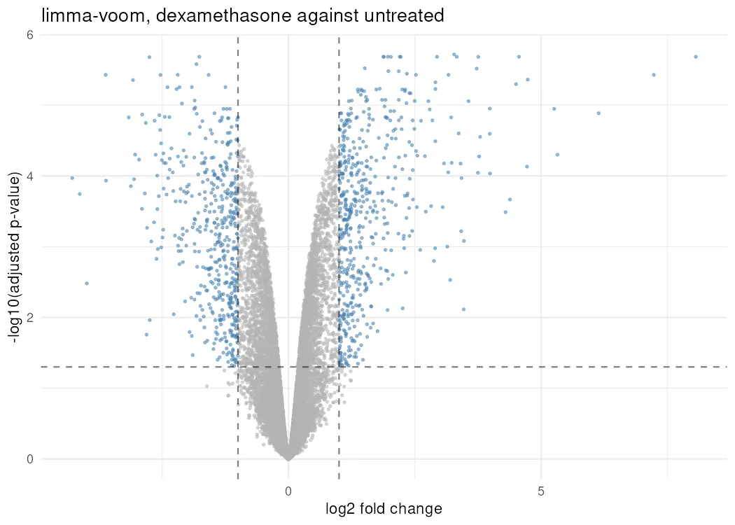

Volcano plot from limma-voom analysis

The volcano plot shows fold change on the x-axis and negative log10 adjusted p-value on the y-axis. Genes in the upper corners are both statistically significant and biologically meaningful. The overall shape is similar to the DESeq2 volcano plot, reflecting the strong agreement between the two methods.

When to choose limma-voom over DESeq2

Both methods are excellent and will give similar results on most datasets. Here are situations where limma-voom has advantages:

Speed. limma is faster than DESeq2 on large datasets with many samples. The linear modeling framework scales well.
Complex designs. limma handles complex experimental designs more naturally. Random effects, interaction terms, and blocking factors are straightforward to specify.
Small sample sizes. The empirical Bayes moderation in limma performs well when you have very few replicates. It borrows strength across genes effectively.
Existing microarray pipelines. If your lab already uses limma for microarray data, extending it to RNA-seq with voom requires minimal code changes.

DESeq2 is preferred when you want built-in shrinkage of log2 fold changes, or when you prefer the negative binomial framework. For most standard analyses, either method works well.

Next: Enrichment