ML Concepts

Machine learning builds models that learn patterns from data. Instead of writing explicit rules, you provide examples and the algorithm finds the rules itself. This page covers the foundations you need before writing any code.

Supervised vs unsupervised learning

Supervised learning uses labeled data: each example has input features and a known output, and the model learns to map inputs to outputs. Examples: predicting tumor malignancy from gene expression, patient survival from clinical variables, cell type from single-cell RNA-seq.

Unsupervised learning uses unlabeled data. There is no target; the model finds structure on its own. Examples: clustering patients into subgroups, reducing high-dimensional data to 2D (PCA, UMAP), finding co-expressed gene modules.

This section focuses on supervised learning for tabular data.

Regression vs classification

Regression predicts a continuous number (drug IC50, patient age, expression level). Classification predicts a category (tumor vs normal, cancer subtype, cell type). The choice determines which algorithms, loss functions, and metrics you use.

The training workflow

1. Split the data into training and test sets. Hold the test set out.
2. Preprocess the training data (scale, encode, impute).
3. Train a model on the training data.
4. Evaluate on the test set to estimate real-world performance.

┌─────────────────────────────────────┐
│           Full dataset              │
├─────────────────────┬───────────────┤
│   Training set      │   Test set    │
│   (fit model)       │   (evaluate)  │
│   ~80%              │   ~20%        │
└─────────────────────┴───────────────┘

Evaluating on the same data you trained on gives an overly optimistic estimate. That is one of the most common mistakes in machine learning.

Bias-variance tradeoff

Model error comes from two sources. Bias is error from oversimplifying: a high-bias model underfits and misses real patterns. Variance is error from being too sensitive to the training data: a high-variance model overfits and captures noise as signal.

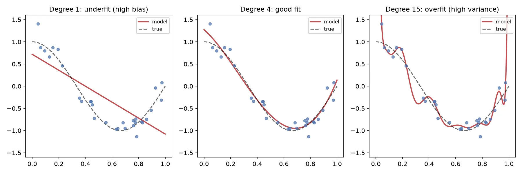
The same noisy data (the dashed line is the truth) fit by three polynomials. Degree 1 is too simple to follow the curve (high bias). Degree 4 tracks it well. Degree 15 wiggles through every point, chasing noise (high variance). Reducing bias increases variance and vice versa; the goal is the sweet spot where total error is lowest.

Overfitting and underfitting

Overfitting: good on training data, poor on new data. The model memorized examples instead of learning generalizable patterns. Signs: training accuracy far above test accuracy, a very complex model.

Underfitting: poor on both training and test data. The model is too simple. Signs: both accuracies low, and adding complexity improves both.

Prevent overfitting with more data, a simpler model, regularization, cross-validation, and early stopping.

Parameters vs hyperparameters

Parameters are learned during training (regression weights, tree split points). Hyperparameters are set before training and control the learning process (number of trees, learning rate, regularization strength, tree depth). Choosing them well is hyperparameter tuning, covered in the Cross-Validation page.

No free lunch

No single algorithm is best for every problem. The right choice depends on dataset size, feature types, whether the relationship is linear, and whether you need interpretability. Compare several algorithms on your data rather than assuming one wins. The Algorithms Overview describes the main ones and when each tends to work.

Next steps

The next page covers EDA: exploring your dataset before building any models.