Compensation

Every fluorophore leaks signal into detectors that belong to other fluorophores. The amount of leakage is the spillover, and it is a property of the instrument and the panel, not of the sample. Compensation subtracts the leaked signal so that a fluorescent signal on one detector reflects only the fluorophore bound to that detector’s antibody.

Why before transformation

Spillover is linear. If fluorophore A spills 10 percent of its signal into detector B, then the correction is a matrix multiplication on the raw intensities. Logicle and arcsinh transforms are nonlinear, and a linear correction applied after a nonlinear transform is no longer the correct correction. The order is fixed: compensate on the linear scale, then transform.

The spillover matrix

The spillover matrix is a square matrix with one row and column per fluorophore. The diagonal is 100, and the off-diagonal entries are the percentage of one fluorophore’s signal that appears in another detector. The instrument writes it into the FCS file under the SPILL keyword, computed from single-stain control tubes at acquisition time.

library(flowCore)

extdata_dir <- system.file("extdata", package = "flowCore")
fcs_files <- list.files(extdata_dir, pattern = "0877408774", full.names = TRUE)
frames <- lapply(fcs_files, read.FCS, transformation = FALSE)

# Find a frame that carries a spillover matrix in its keywords.
#' Read the spillover matrix keyword from a flowFrame.
#'
#' @param frame A `flowFrame`.
#' @return The spillover matrix, or NULL when the keyword is absent.
SpillKey <- function(frame) {
  value <- keyword(frame, "SPILL")[[1]]
  if (is.null(value) || length(value) == 0) {
    value <- keyword(frame, "$SPILLOVER")[[1]]
  }
  value
}
has_spill <- vapply(frames, function(f) !is.null(SpillKey(f)), logical(1))
frame <- frames[[1]]

if (any(has_spill)) {
  spill <- flowCore::spillover(frame)$SPILL
} else {
  # No stored matrix: load one computed from single-stain controls that
  # ship with flowCore for this teaching panel.
  comp_path <- file.path(extdata_dir, "compdata", "compmatrix")
  lines <- readLines(comp_path)
  lines <- lines[nzchar(lines)]
  chan <- strsplit(lines[3], "\t")[[1]]
  spill <- do.call(rbind, lapply(lines[4:length(lines)], function(l) {
    as.numeric(strsplit(l, "\t")[[1]])
  }))
  colnames(spill) <- chan
  rownames(spill) <- chan
}

spill

         FL1-H    FL2-H   FL3-H   FL4-H
FL1-H 1.000000 0.240000 0.03200 0.00113
FL2-H 0.007770 1.000000 0.14000 0.00274
FL3-H 0.008690 0.170000 1.00000 0.21000
FL4-H 0.000795 0.000995 0.00323 1.00000

The bundled files ship without a stored matrix, so the example loads one that flowCore computed from single-stain controls for this panel. In a real analysis you read the matrix from the keyword, where the instrument wrote it, or compute it from single-stain controls with flowCore::spillover().

Apply the matrix

Compensation is a matrix multiplication. flowCore provides the compensate() generic, which works on a flowFrame or a flowSet and uses the spillover matrix to correct every event.

# Compensate the frame using the matrix above.
compensated <- compensate(frame, spill)

# The first rows before and after correction.
head(exprs(frame)[, colnames(spill)], 3)
head(exprs(compensated)[, colnames(spill)], 3)

     FL1-H FL2-H FL3-H FL4-H
[1,]   618     0   225   286
[2,]   245   431   259   371
[3,]   699   448   215   638
        FL1-H     FL2-H    FL3-H    FL4-H
[1,] 617.2638 -187.6063 230.7458 237.3599
[2,] 240.3468  338.5048 202.8614 327.2000
[3,] 695.1962  254.1646 155.2200 603.9218

The corrected values are smaller on the off-diagonal detectors, because the leaked signal has been subtracted. The diagonal signal, the true measurement, is preserved.

Before and after

The numbers above show the correction on three events. The figure shows it on all ten thousand, which is where you can judge whether the matrix did the right thing.

library(ggplot2)

dir.create("outputs", showWarnings = FALSE, recursive = TRUE)

#' Put two channels of a frame into a plain data frame for plotting.
#'
#' @param frame A `flowFrame`.
#' @param state A label for the compensation state, used as a facet title.
#' @return A data frame with the two channel columns and the state label.
ChannelPair <- function(frame, state) {
  values <- as.data.frame(exprs(frame)[, c("FL1-H", "FL2-H")])
  names(values) <- c("fl1", "fl2")
  values$state <- state
  values
}

pair <- rbind(
  ChannelPair(frame, "raw"),
  ChannelPair(compensated, "compensated")
)
pair$state <- factor(pair$state, levels = c("raw", "compensated"))

comp_plot <- ggplot(pair, aes(x = fl1, y = fl2)) +
  geom_hex(bins = 70) +
  facet_wrap(~state) +
  labs(title = "FL1-H against FL2-H", x = "FL1-H", y = "FL2-H")

ggsave("outputs/cyto-compensation.png", plot = comp_plot,
       width = 8, height = 4, dpi = 110, bg = "white")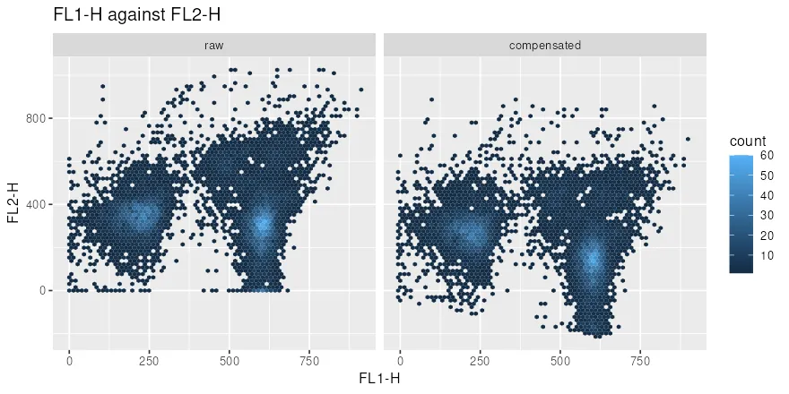

The FL1 dim population barely moves, and the FL1 bright population drops on the FL2 axis. That asymmetry is the whole mechanism, because the subtraction is proportional to the FL1 signal. Part of the corrected population now sits below zero, which is correct behaviour rather than a bug: subtracting a spillover estimate from a noisy count has to produce negative values for cells that were truly negative, and a transformation that cannot represent them will hide the very events that show the correction worked.

The spreading error

A compensated signal carries a spread, not a fixed offset, because the spillover is subtracted from a noisy count. A 10 percent spillover from a bright fluorophore into a dim one can add more variance to the dim channel than its own signal carries. This is the spreading error, and it is why panel design matters: a bright fluorophore placed on a dim marker, spilling into the detector for a bright marker, ruins the dim one. The transformation and QC page picks up from the compensated object.