Over-Representation Analysis

Over-Representation Analysis asks a simple question. You have a list of significant genes. Are any biological pathways or GO terms overrepresented in that list compared to what you would expect by chance?

ORA is the oldest and most widely used pathway analysis method. It works by comparing your gene list against a background set using a statistical test. If a pathway has more of your significant genes than expected, that pathway is enriched.

How ORA works

The logic is straightforward. You start with two sets of genes:

1. Foreground: your significant differentially expressed genes
2. Background: all genes you tested

For each pathway or GO term, ORA builds a 2x2 contingency table. It counts how many foreground genes are in the pathway versus how many are not. Then it compares this to the same ratio in the background. A hypergeometric test or Fisher’s exact test determines whether the overlap is greater than chance.

ORA vs GSEA

ORA requires a hard cutoff to define your significant genes. This is its main limitation. Genes just below the cutoff are discarded entirely. A gene with padj = 0.051 contributes nothing, while a gene with padj = 0.049 contributes equally to one with padj = 1e-100.

Feature	ORA	GSEA
Input	Significant genes only	All genes, ranked
Requires cutoff	Yes	No
Uses magnitude of change	No	Yes
Simple to explain	Yes	Moderate
Risk of missing subtle signals	Higher	Lower

GSEA is generally preferred because it uses more information. ORA is still useful when you have a clear set of hits from an experiment. It is also easier to explain to collaborators who are not familiar with enrichment statistics.

Setup

clusterProfiler runs the enrichment in R and gseapy does the same job in Python. Both tabs below work from one DESeq2 result and one set of GO definitions, so the two answers are comparable.

The page recomputes the differential expression rather than reading a file, so it stands on its own.

library(tidyverse)
library(clusterProfiler)
library(org.Hs.eg.db)
library(GO.db)
library(DESeq2)
library(airway)

data("airway")
dds <- DESeqDataSet(airway, design = ~ cell + dex)
dds$dex <- relevel(dds$dex, ref = "untrt")
dds <- dds[rowSums(counts(dds)) >= 10, ]
dds <- DESeq(dds)

res <- as.data.frame(results(dds, contrast = c("dex", "trt", "untrt")))
res$gene <- rownames(res)
nrow(res)

[1] 22369

Define significant genes

We apply a standard cutoff: adjusted p-value < 0.05 and absolute log2 fold change > 1. This selects genes that are both statistically significant and biologically meaningful.

R

sig_genes <- res |>
  filter(padj < 0.05, abs(log2FoldChange) > 1) |>
  pull(gene)

bg_genes <- res |>
  filter(!is.na(padj)) |>
  pull(gene)

length(sig_genes)
length(bg_genes)

# Hand both lists, and the GO definitions, to the Python tab. Restricting the
# terms to a usable size range is the same filter enrichGO applies internally.
dir.create("outputs", showWarnings = FALSE, recursive = TRUE)
writeLines(sig_genes, "outputs/ora_significant.txt")
writeLines(bg_genes, "outputs/ora_background.txt")

go_map <- AnnotationDbi::select(
  org.Hs.eg.db,
  keys = bg_genes,
  columns = c("GO", "ONTOLOGY"),
  keytype = "ENSEMBL"
)
# Bioconductor attaches a dplyr::count() of its own, so name dplyr's explicitly.
go_map <- go_map |>
  dplyr::filter(!is.na(GO), ONTOLOGY == "BP") |>
  dplyr::distinct(GO, ENSEMBL)

go_sizes <- dplyr::count(go_map, GO)
keep_terms <- go_sizes |>
  dplyr::filter(n >= 10, n <= 500) |>
  dplyr::pull(GO)
go_map <- go_map |> dplyr::filter(GO %in% keep_terms)
# Carry the term names too, so the Python tab can print something readable.
go_names <- AnnotationDbi::select(
  GO.db, keys = keep_terms, columns = "TERM", keytype = "GOID"
)
go_map <- go_map |>
  dplyr::left_join(go_names, by = c("GO" = "GOID"))

write_csv(go_map, "outputs/ora_go_sets.csv")
length(keep_terms)

[1] 1018
[1] 18032
[1] 2065

Python

import pandas as pd
import gseapy as gp

significant = pd.read_csv(
    "outputs/ora_significant.txt", header=None
)[0].tolist()
background = pd.read_csv(
    "outputs/ora_background.txt", header=None
)[0].tolist()

go_sets = pd.read_csv("outputs/ora_go_sets.csv")
names = dict(zip(go_sets["GO"], go_sets["TERM"]))
gene_sets = go_sets.groupby("GO")["ENSEMBL"].apply(list).to_dict()

print(len(significant))
print(len(background))
print(len(gene_sets))

1018
18032
2065

[1] 999
[1] 17165

We have 999 significant DEGs out of 17,165 tested genes.

Convert gene IDs

GO and KEGG analyses in clusterProfiler require Entrez gene IDs. Our DESeq2 results use Ensembl IDs. The bitr() function handles the conversion.

sig_entrez <- bitr(
  sig_genes,
  fromType = "ENSEMBL",
  toType = "ENTREZID",
  OrgDb = org.Hs.eg.db
)

bg_entrez <- bitr(
  bg_genes,
  fromType = "ENSEMBL",
  toType = "ENTREZID",
  OrgDb = org.Hs.eg.db
)

nrow(sig_entrez)
nrow(bg_entrez)

[1] 949
[1] 15273

The conversion mapped 938 of 999 significant genes and 14,761 of 17,165 background genes. Some Ensembl IDs do not have corresponding Entrez IDs. This is normal and the loss is small.

GO enrichment

Gene Ontology groups genes into three categories: Biological Process, Molecular Function, and Cellular Component. Biological Process is the most commonly used for pathway-level interpretation.

R

ego <- enrichGO(
  gene = sig_entrez$ENTREZID,
  universe = bg_entrez$ENTREZID,
  OrgDb = org.Hs.eg.db,
  ont = "BP",
  pAdjustMethod = "BH",
  pvalueCutoff = 0.05,
  readable = TRUE
)

ego |>
  as_tibble() |>
  dplyr::select(Description, GeneRatio, p.adjust, Count) |>
  head(10)

# A tibble: 10 × 4
   Description                     GeneRatio   p.adjust Count
   <chr>                           <chr>          <dbl> <int>
 1 circulatory system process      58/814    0.00000124    58
 2 regulation of system process    54/814    0.00000198    54
 3 vasculature development         68/814    0.00000198    68
 4 blood circulation               49/814    0.00000200    49
 5 regulation of blood circulation 32/814    0.00000583    32
 6 blood vessel development        64/814    0.00000699    64
 7 axon guidance                   29/814    0.00000866    29
 8 neuron projection guidance      29/814    0.00000901    29
 9 animal organ morphogenesis      58/814    0.0000174     58
10 angiogenesis                    56/814    0.0000181     56

Python

ora_res = gp.enrich(
    gene_list=significant,
    gene_sets=gene_sets,
    background=background,
    outdir=None,
)

results = ora_res.results.sort_values("Adjusted P-value")
results["Description"] = results["Term"].map(names)
columns = ["Description", "Overlap", "Adjusted P-value"]
print(results[columns].head(10).to_string(index=False))

                                                    Description Overlap  Adjusted P-value
                                                  cell adhesion  57/432          0.000003
                                                  axon guidance  24/113          0.000010
                                                   angiogenesis  33/200          0.000012
                                     nervous system development  55/449          0.000018
                                            cell-cell signaling  21/104          0.000082
                          positive regulation of cell migration  32/213          0.000092
cell surface receptor protein tyrosine kinase signaling pathway   18/84          0.000163
                              intracellular signal transduction  47/393          0.000167
                   G protein-coupled receptor signaling pathway  35/257          0.000193
                                                immune response  27/177          0.000296

# A tibble: 10 × 4
   Description                                   GeneRatio      p.adjust Count
   <chr>                                         <chr>             <dbl> <int>
 1 regulation of system process                  62/807    0.00000000622    62
 2 circulatory system process                    65/807    0.0000000493     65
 3 muscle system process                         52/807    0.000000127      52
 4 blood circulation                             56/807    0.000000168      56
 5 axon guidance                                 35/807    0.000000168      35
 6 neuron projection guidance                    35/807    0.000000168      35
 7 extracellular matrix organization             45/807    0.000000898      45
 8 extracellular structure organization          45/807    0.000000898      45
 9 external encapsulating structure organization 45/807    0.000000942      45
10 blood vessel morphogenesis                    69/807    0.000000942      69

The GeneRatio column shows how many significant genes belong to each term out of the total mapped genes.

The two tabs do not return the same ranking, and the reason is the gene sets rather than the test. enrichGO walks the GO graph, so a gene annotated to a specific child term also counts toward every parent above it. The sets exported for the Python tab hold direct annotations only, which makes each set smaller and shifts which ones clear the correction. Both find the same biology, the vascular and axon guidance and adhesion terms, and neither ordering is the right one to quote without saying which gene sets produced it.

GO dot plot

The dot plot shows the top enriched GO terms. Dot size represents gene count. Color represents adjusted p-value.

dot_plot <- dotplot(ego, showCategory = 15) + theme_minimal()
ggsave("outputs/ora-go-dotplot.png", dot_plot,
       width = 8, height = 7, dpi = 110, bg = "white")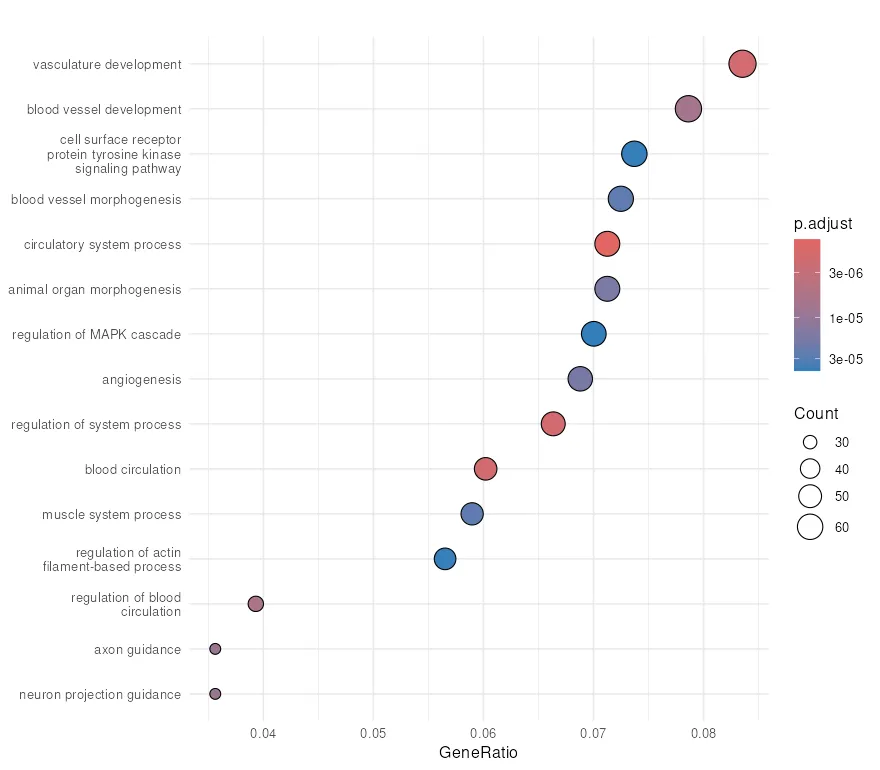

Larger, darker dots indicate terms with many genes and strong statistical significance. Blood vessel morphogenesis has the highest gene count at 69. Regulation of system process has the lowest adjusted p-value.

GO bar plot

A bar plot provides an alternative view. It ranks terms by gene count.

bar_plot <- barplot(ego, showCategory = 15) + theme_minimal()
ggsave("outputs/ora-go-barplot.png", bar_plot,
       width = 8, height = 7, dpi = 110, bg = "white")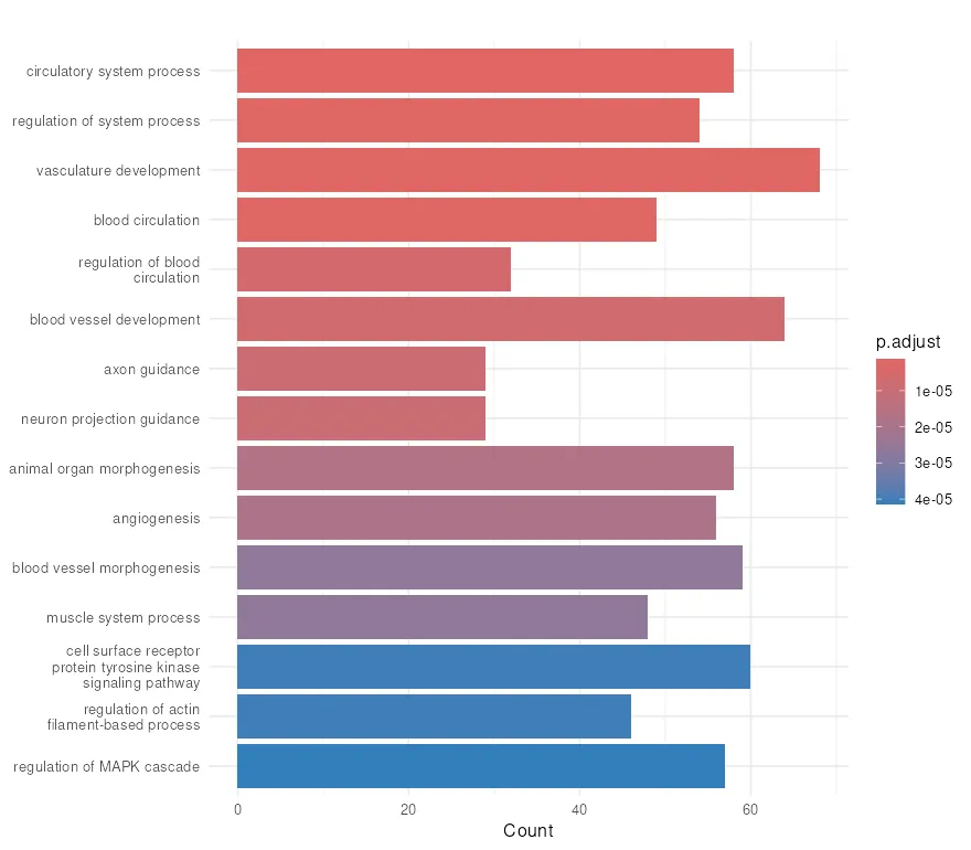

KEGG pathway enrichment

Reference only

enrichKEGG queries the KEGG web service when it runs, so its answer holds only until that database changes underneath it. The block below is not executed by this page’s container run, and it is the one place on the page where the output is not reproducible from the image. Everything above it is.

ekegg <- enrichKEGG(
  gene = sig_entrez$ENTREZID,
  universe = bg_entrez$ENTREZID,
  organism = "hsa",
  pvalueCutoff = 0.05
)

ekegg |>
  as_tibble() |>
  dplyr::select(Description, GeneRatio, p.adjust, Count) |>
  head(10)

# A tibble: 10 × 4
   Description                                      GeneRatio  p.adjust Count
   <chr>                                            <chr>         <dbl> <int>
 1 Cytokine-cytokine receptor interaction           29/455    0.0000555    29
 2 Regulation of lipolysis in adipocytes            15/455    0.0000555    15
 3 Inflammatory mediator regulation of TRP channels 18/455    0.000987     18
 4 Tyrosine metabolism                              9/455     0.00184       9
 5 Cytoskeleton in muscle cells                     30/455    0.00184      30
 6 Axon guidance                                    27/455    0.00198      27
 7 Hormone signaling                                20/455    0.00700      20
 8 Neuroactive ligand-receptor interaction          20/455    0.0130       20
 9 Retinol metabolism                               8/455     0.0163        8
10 Circadian entrainment                            13/455    0.0275       13

Export results

ego |>
  as_tibble() |>
  write_csv("outputs/ora_go_results.csv")

Summary

ORA tests whether specific pathways are overrepresented among your significant genes. In the airway dataset, we found 999 significant DEGs. GO analysis revealed enrichment in system regulation, circulatory processes, and extracellular matrix organization. KEGG analysis highlighted cytokine signaling and lipolysis regulation. These results confirm that dexamethasone treatment broadly affects inflammatory and metabolic pathways.

Next: Gene Set Enrichment Analysis (GSEA)