Logistic Regression

When the outcome is yes or no, responder or not, alive or dead, linear regression is the wrong tool. It would predict probabilities below zero and above one. Logistic regression models the probability directly and reports its effects as odds ratios, the currency of clinical papers. This page predicts treatment response from a biomarker, in R and Python.

Every code block on this page runs in a container in the companion repository. The numbers and figure come from those real runs.

When to use logistic regression

Use it whenever the outcome is binary. It models the log-odds of the outcome as a linear function of the predictors, so the probability always stays between zero and one. The coefficients become odds ratios once exponentiated.

The data

logistic.csv has 120 patients with a continuous biomarker and a binary responder outcome.

R

df <- read.csv("logistic.csv")

Python

import pandas as pd

df = pd.read_csv("logistic.csv")

Fitting the model

R

fit <- glm(responder ~ biomarker, data = df, family = binomial)
summary(fit)

            Estimate Std. Error z value Pr(>|z|)
(Intercept)  -4.6123     0.8917  -5.173 2.31e-07 ***
biomarker     1.0587     0.1925   5.501 3.78e-08 ***

Python

import statsmodels.formula.api as smf

model = smf.logit("responder ~ biomarker", data=df).fit()
model.summary()

                 coef    std err          z      P>|z|
Intercept     -4.6123      0.892     -5.172      0.000
biomarker      1.0587      0.192      5.500      0.000

The biomarker coefficient is 1.06 on the log-odds scale, and clearly non-zero. But log-odds are hard to read. Odds ratios are the natural language.

Odds ratios

Exponentiate a coefficient to turn it into an odds ratio.

R

exp(cbind(OR = coef(fit), confint.default(fit)))

               OR 2.5 % 97.5 %
(Intercept) 0.010 0.002  0.057
biomarker   2.883 1.977  4.203

Python

import numpy as np

np.exp(model.params)
np.exp(model.conf_int())

              OR   2.5%  97.5%
biomarker  2.883  1.977  4.204

The odds ratio for the biomarker is 2.88, with a confidence interval from 1.98 to 4.20. Each one-unit rise in the biomarker nearly triples the odds of responding. The interval excludes 1, so the effect is significant. Both languages agree.

The logistic curve

Plotting the predicted probability against the biomarker gives the familiar S-curve. It rises from near zero to near one, steepest in the middle.

R

library(ggplot2)

ggplot(df, aes(biomarker, responder)) +
  geom_point(alpha = 0.3) +
  geom_smooth(method = "glm", method.args = list(family = binomial))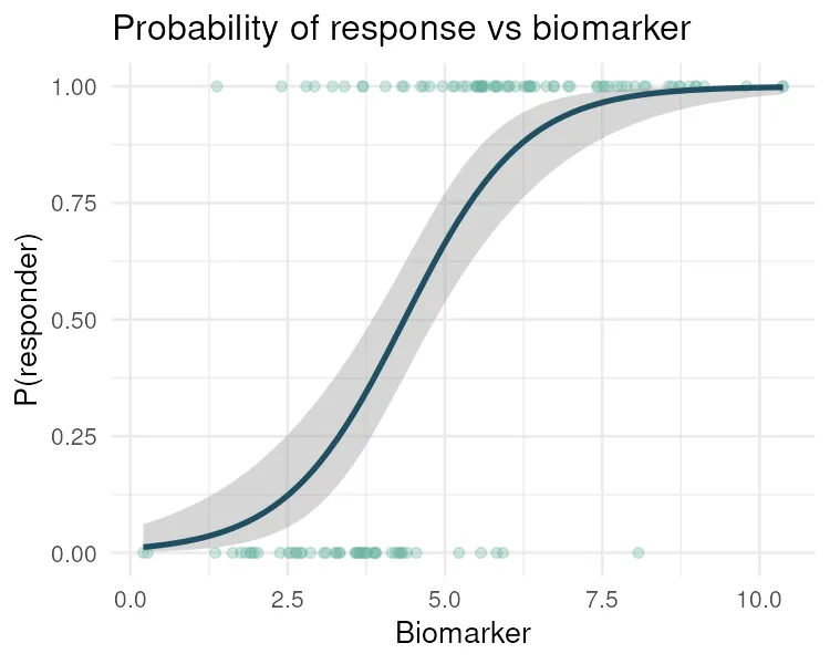

Python

xs = np.linspace(df["biomarker"].min(), df["biomarker"].max(), 200)
pred = model.predict(pd.DataFrame({"biomarker": xs}))
plt.scatter(df["biomarker"], df["responder"], alpha=0.3)
plt.plot(xs, pred)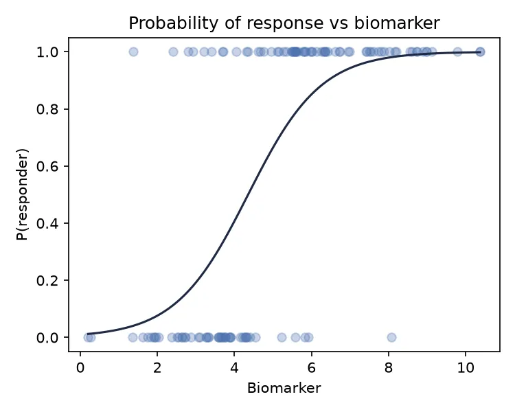

Pitfalls and bioinformatics notes

• An odds ratio is not a risk ratio. For common outcomes the odds ratio exaggerates the risk ratio. Say “odds”, not “times more likely”, unless the outcome is rare.
• Coefficients are log-odds, not probabilities. Always exponentiate for interpretation, and remember the effect on probability depends on where you start on the curve.
• Watch for separation. If a predictor perfectly splits the outcome, the model fails to converge and coefficients blow up. Small or imbalanced datasets are prone to it.
• Enough events per predictor. A rough rule is at least ten outcome events per predictor. Fewer, and the estimates are unstable.

Key points

• Logistic regression models a binary outcome and keeps predictions between zero and one.
• Exponentiate the coefficients to get odds ratios, the standard clinical effect measure.
• An odds ratio whose confidence interval excludes 1 is significant.
• Odds ratios are not risk ratios unless the outcome is rare.

Further reading

• STHDA, logistic regression.
• An Introduction to Statistical Learning, chapter 4.
• The next guide, ROC curves and AUC, which measures how well such a model classifies.