Enrichment

A differential expression table ends with a list of genes, and the next question is whether that list is enriched for a biological process. There are two ways to ask. Over-representation analysis takes the genes that pass a significance cutoff and asks which annotated terms appear in the list more often than chance. Gene set enrichment analysis skips the cutoff, works from the ranked list of every tested gene, and asks whether a term’s genes gather at one end of the ranking. The two tests answer different questions, so a full analysis runs both.

Both run here through clusterProfiler, which is the route the Practical Bioinformatics chapter behind this section teaches, and the one most published analyses use.

The results, recomputed

The page is self-contained, so it recomputes the DESeq2 result. It keeps two versions of it. The shrunken table carries the fold changes, and the unshrunken one carries the Wald statistic, because lfcShrink() replaces the fold change and drops the stat column with it.

library(DESeq2)
library(airway)
library(dplyr)
library(clusterProfiler)
library(org.Hs.eg.db)
library(enrichplot)
library(ggplot2)

data(airway)
dds <- DESeqDataSet(airway, design = ~ cell + dex)
dds$dex <- relevel(dds$dex, ref = "untrt")
dds <- dds[rowSums(counts(dds)) >= 10, ]
dds <- DESeq(dds)

res_shrunk <- lfcShrink(dds, coef = "dex_trt_vs_untrt", type = "apeglm")
results_df <- as.data.frame(res_shrunk)
results_df$gene_id <- rownames(results_df)

res_wald <- as.data.frame(results(dds, name = "dex_trt_vs_untrt"))
res_wald$gene_id <- rownames(res_wald)

# The upregulated significant genes, as Ensembl IDs.
sig_up <- results_df |>
  filter(padj < 0.05, log2FoldChange > 0) |>
  pull(gene_id)
length(sig_up)

[1] 2193

Mapping the identifiers

The airway rows are Ensembl IDs and the annotation databases are keyed on Entrez. bitr converts between them, and the count that comes out is worth reading rather than ignoring.

entrez_up <- bitr(
  sig_up,
  fromType = "ENSEMBL",
  toType = "ENTREZID",
  OrgDb = org.Hs.eg.db
)

# Genes in, genes mapped.
length(sig_up)
nrow(entrez_up)

[1] 2193
[1] 2091

Some Ensembl genes have no Entrez equivalent, so no tool keyed on Entrez can test them. They leave the analysis here, and nothing downstream will mention them again.

Over-representation

enrichGO runs the hypergeometric test over GO Biological Process terms and applies Benjamini-Hochberg correction. readable = TRUE puts gene symbols in the result instead of Entrez IDs.

go_bp <- enrichGO(
  gene = entrez_up$ENTREZID,
  OrgDb = org.Hs.eg.db,
  ont = "BP",
  pAdjustMethod = "BH",
  pvalueCutoff = 0.05,
  readable = TRUE
)

go_df <- as.data.frame(go_bp)

# Terms passing the cutoff, then the strongest six.
nrow(go_df)
head(go_df[, c("Description", "GeneRatio", "pvalue", "p.adjust")], 6)

[1] 536
                                             Description GeneRatio       pvalue
GO:0007015                   actin filament organization  102/1869 5.378504e-16
GO:0071375 cellular response to peptide hormone stimulus   77/1869 2.480673e-13
GO:0043434                   response to peptide hormone   92/1869 4.725783e-13
GO:0032970    regulation of actin filament-based process   84/1869 1.172761e-12
GO:0031589                       cell-substrate adhesion   76/1869 2.648946e-12
GO:0032956 regulation of actin cytoskeleton organization   71/1869 4.176105e-10
               p.adjust
GO:0007015 2.922679e-12
GO:0071375 6.739989e-10
GO:0043434 8.559968e-10
GO:0032970 1.593196e-09
GO:0031589 2.878874e-09
GO:0032956 3.782159e-07

GeneRatio is the fraction of the submitted genes that carry the term. A term matters when that fraction sits far above what the term’s size in the background would predict, and the p-value is the measure of how far.

dir.create("outputs", showWarnings = FALSE, recursive = TRUE)

ora_plot <- dotplot(go_bp, showCategory = 12) +
  labs(title = "GO biological process, upregulated genes")

ggsave("outputs/rnaseq-ora-dotplot.png", ora_plot,
       width = 7, height = 6, dpi = 110, bg = "white")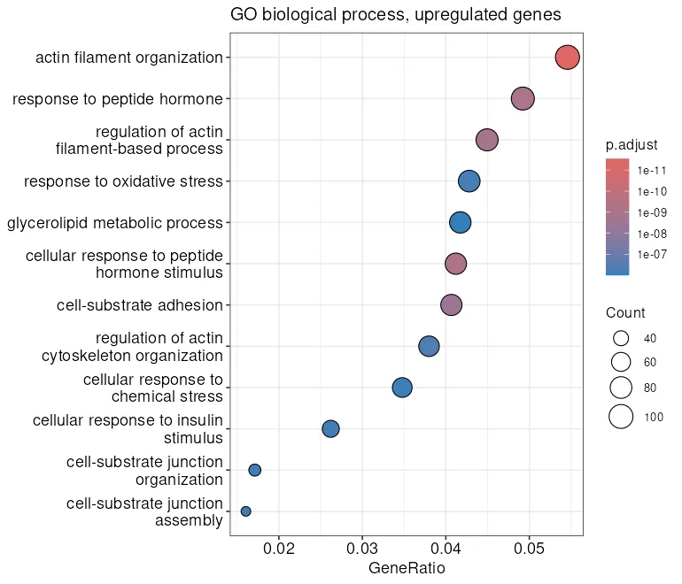

Actin organization at the top of a glucocorticoid experiment in airway smooth muscle is the expected answer, and seeing it is the point of running the test on a dataset whose biology is already known.

GSEA, and what the ranking is worth

GSEA needs one number per gene that carries both the direction of the change and its significance. The chapter ranks by the signed negative log p-value of the shrunken table. The Wald statistic from results() is the other candidate. They are not equivalent, and the gap is large enough to measure rather than argue about.

#' Map a ranked gene table to Entrez and run gseGO on the ranking.
#'
#' @param ranked A data frame with a gene_id column and a rank column, sorted
#'   with the largest rank first.
#' @return A `gseaResult` with the terms passing the adjusted p-value cutoff.
RunGseGo <- function(ranked) {
  mapped <- bitr(ranked$gene_id, fromType = "ENSEMBL", toType = "ENTREZID",
                 OrgDb = org.Hs.eg.db)
  joined <- ranked |>
    inner_join(mapped, by = c("gene_id" = "ENSEMBL")) |>
    distinct(ENTREZID, .keep_all = TRUE)
  gene_list <- sort(setNames(joined$rank, joined$ENTREZID), decreasing = TRUE)
  set.seed(1)
  gseGO(geneList = gene_list, OrgDb = org.Hs.eg.db, ont = "BP",
        minGSSize = 10, maxGSSize = 500, pvalueCutoff = 0.05,
        verbose = FALSE, seed = TRUE)
}

# The chapter's ranking, signed -log10(p) on the shrunken table.
signed_log_p <- results_df |>
  filter(!is.na(pvalue), !is.na(log2FoldChange)) |>
  mutate(rank = sign(log2FoldChange) * -log10(pvalue)) |>
  arrange(desc(rank))

# The Wald statistic, from the unshrunken table.
wald <- res_wald |>
  filter(!is.na(stat)) |>
  mutate(rank = stat) |>
  arrange(desc(rank))

gsea_signed <- RunGseGo(signed_log_p)
gsea_wald <- RunGseGo(wald)

# Terms passing the cutoff under each ranking.
nrow(as.data.frame(gsea_signed))
nrow(as.data.frame(gsea_wald))

[1] 435
[1] 975

Both rankings work, and the Wald statistic finds more than twice as many terms. The signed negative log p-value discards the size of the effect and keeps only its direction and its certainty, so a gene that barely moved but moved reliably ranks beside a gene that doubled.

gsea_df <- as.data.frame(gsea_wald)
head(gsea_df[, c("Description", "NES", "pvalue", "p.adjust")], 6)

                                                         Description       NES
GO:0050951                sensory perception of temperature stimulus -2.082983
GO:0071276                          cellular response to cadmium ion  2.041477
GO:0098704                carbohydrate import across plasma membrane  2.027693
GO:0098708                   D-glucose import across plasma membrane  2.027693
GO:0140271                      hexose import across plasma membrane  2.027693
GO:1900024 regulation of substrate adhesion-dependent cell spreading  2.018185
                 pvalue    p.adjust
GO:0050951 4.387203e-05 0.007449753
GO:0071276 1.297378e-05 0.006195737
GO:0098704 1.647802e-05 0.006195737
GO:0098708 1.647802e-05 0.006195737
GO:0140271 1.647802e-05 0.006195737
GO:1900024 1.986470e-05 0.006268920

A positive normalized enrichment score puts the term’s genes at the top of the ranking, the upregulated end. A negative one puts them at the bottom.

Those six terms are also a warning about reading a GSEA table from the top. With 975 terms below the cutoff, sorting by p-value favours small, narrowly defined sets, which is why cadmium ion and temperature perception appear ahead of anything a reader would call the headline result. The over-representation dot plot above is the interpretable view of the same data, and sorting the GSEA table by the enrichment score rather than the p-value gives the same kind of answer.

gsea_plot <- gseaplot2(gsea_wald, geneSetID = 1:3)

ggsave("outputs/rnaseq-gsea-plot.png", gsea_plot,
       width = 8, height = 6, dpi = 110, bg = "white")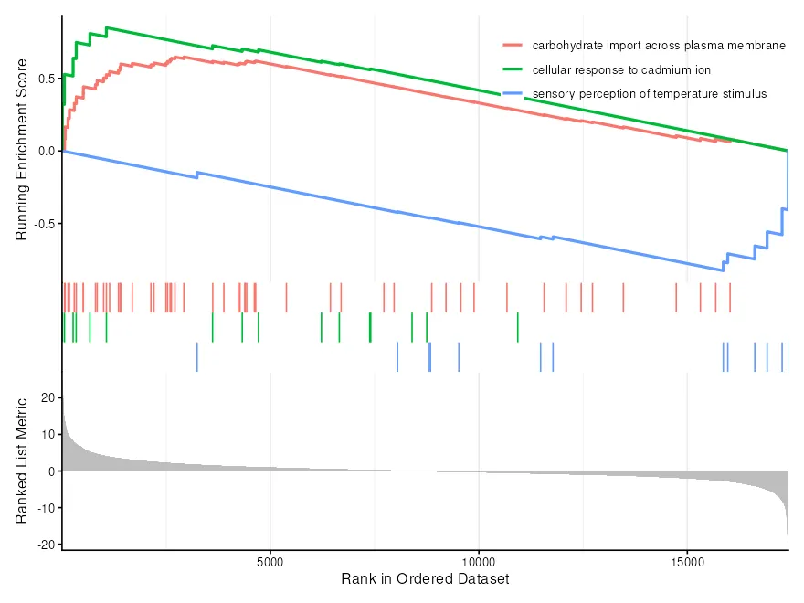

KEGG and Reactome

enrichKEGG and the Reactome equivalents query a web service when they run. They are the right next step when GO is too coarse for the question, and they are also the reason this page stops at GO. A pinned container cannot pin the contents of a remote database, so a KEGG result holds only until that database changes underneath it, while this section promises that every number here comes back from the container that produced it.

The pipeline route in the nf-core differential abundance guide runs the pathway step and records the database version it used, which is the reproducible way to get the same answer twice.