Automated Gating

The previous page drew a boundary by hand and applied the same boundary to a second sample, where it did not belong. Automated gating keeps the hierarchy and moves the boundary. The template names the channel and the method for each gate, and each sample’s own distribution decides where the cut goes.

The template is a CSV, and that is the part worth noticing. A gate drawn with a mouse lives inside a workspace file, where no reviewer can read it and no version control system can show what changed between two analyses. A template is a text file with one row per gate, so a changed method shows up in a diff the way a changed line of code does.

The template

One row per population. alias names it, parent says which population it is measured within, dims names the channel to cut on, and gating_method names the algorithm that finds the cut.

# The template ships beside this guide's code, so the page prints the file the
# gating step actually reads.
template_path <- "gating_template.csv"
cat(readLines(template_path), sep = "\n")

alias,pop,parent,dims,gating_method,gating_args,collapseDataForGating,groupBy,preprocessing_method,preprocessing_args
CD45,+,root,CD45,mindensity,,,,,
CD3,+,CD45,CD3,mindensity,,,,,
CD4,+,CD3,CD4,mindensity,,,,,
CD20,+,CD45,CD20,mindensity,,,,,

mindensity puts the boundary at the lowest point of the density between two modes, which is the automated version of what a person does by eye. The deposited PBMC template in the everything-flow-cytometry repository starts with flowClust on FSC-A and SSC-A to drop debris and singletGate on FSC-A against FSC-H to drop doublets. This panel is mass cytometry, so it has neither channel, and the hierarchy starts at CD45.

Running it

gatingTemplate parses the CSV, GatingSet wraps the data, and gt_gating fits every gate in the template to every sample.

library(flowCore)
library(flowWorkspace)
library(openCyto)
library(HDCytoData)

fs <- Bodenmiller_BCR_XL_flowSet()[1:2]

# Arcsinh transform the surface markers, cofactor 5, then shorten the channel
# names to the bare marker so the template's dims column can name them.
cd_channels <- grep("^CD", colnames(fs), value = TRUE)
asinh_trans <- arcsinhTransform(a = 0, b = 1 / 5, c = 0)
fs <- transform(fs, transformList(cd_channels, tfun = asinh_trans))
colnames(fs) <- sub("\\(.*$", "", colnames(fs))

template <- gatingTemplate(template_path)
gs <- GatingSet(fs)

# One core, because a failed gate is easier to read without parallel output.
gt_gating(template, gs, mc.cores = 1, parallel_type = "none")
recompute(gs)

# The populations the template produced, as paths.
gs_get_pop_paths(gs)

[1] "root"          "/CD45"         "/CD45/CD20"    "/CD45/CD3"
[5] "/CD45/CD3/CD4"

The counts

gs_pop_get_stats returns one row per sample and population. The percentage is of the parent population, which is the number a paper reports.

percents <- as.data.frame(gs_pop_get_stats(gs, type = "percent"))
percents$percent <- round(100 * percents$percent, 1)
percents

                               sample           pop percent
1     PBMC8_30min_patient1_BCR-XL.fcs          root   100.0
2     PBMC8_30min_patient1_BCR-XL.fcs         /CD45    98.5
3     PBMC8_30min_patient1_BCR-XL.fcs    /CD45/CD20    95.3
4     PBMC8_30min_patient1_BCR-XL.fcs     /CD45/CD3    84.0
5     PBMC8_30min_patient1_BCR-XL.fcs /CD45/CD3/CD4    29.9
6  PBMC8_30min_patient1_Reference.fcs          root   100.0
7  PBMC8_30min_patient1_Reference.fcs         /CD45    97.7
8  PBMC8_30min_patient1_Reference.fcs    /CD45/CD20   100.0
9  PBMC8_30min_patient1_Reference.fcs     /CD45/CD3    82.3
10 PBMC8_30min_patient1_Reference.fcs /CD45/CD3/CD4    42.7

Three of the four gates behave. CD45 keeps almost everything, which is right for a leukocyte preparation. CD3 lands near 84 and 82 percent of CD45, and CD4 splits the T cells differently in the two samples, which is the behaviour the template exists for.

The CD20 gate is wrong. It calls 95.3 percent of leukocytes B cells in one sample and 100 percent in the other, and a PBMC sample is not almost entirely B cells.

Why that gate failed

mindensity looks for a valley between two modes. CD20 in this panel does not have one. Almost every event sits in a negative peak near zero, with a thin positive tail, so there is no minimum to find and the method puts the boundary below the whole distribution.

cd20 <- exprs(fs[[1]])[, "CD20"]

# The distribution the gate had to work with.
round(quantile(cd20, c(0.5, 0.75, 0.9, 0.95, 0.99)), 2)

# CD3 for contrast: a marker that does separate into two groups.
round(quantile(exprs(fs[[1]])[, "CD3"], c(0.5, 0.75, 0.9, 0.95, 0.99)), 2)

  50%   75%   90%   95%   99%
-0.09 -0.02  0.93  2.63  5.03
 50%  75%  90%  95%  99%
2.60 3.27 3.77 4.00 4.38

The median CD20 event and the event at the 75th percentile are both negative, while the CD3 median already sits well above zero. CD3 is bimodal and CD20 is a tail, and a method that hunts for a valley cannot tell you that.

Constraining the search

openCyto takes arguments per row. Telling mindensity to look only above 2 stops it from placing the cut under the negative peak.

constrained_path <- "gating_template_constrained.csv"
cat(readLines(constrained_path), sep = "\n")

gs2 <- GatingSet(fs)
gt_gating(gatingTemplate(constrained_path), gs2, mc.cores = 1,
          parallel_type = "none")
recompute(gs2)

cd20_stats <- as.data.frame(gs_pop_get_stats(gs2, type = "percent"))
cd20_stats <- cd20_stats[grepl("CD20", cd20_stats$pop), ]
cd20_stats$percent <- round(100 * cd20_stats$percent, 1)
cd20_stats

alias,pop,parent,dims,gating_method,gating_args,collapseDataForGating,groupBy,preprocessing_method,preprocessing_args
CD45,+,root,CD45,mindensity,,,,,
CD3,+,CD45,CD3,mindensity,,,,,
CD4,+,CD3,CD4,mindensity,,,,,
CD20,+,CD45,CD20,mindensity,min=2,,,,
                              sample        pop percent
3    PBMC8_30min_patient1_BCR-XL.fcs /CD45/CD20     6.2
8 PBMC8_30min_patient1_Reference.fcs /CD45/CD20    22.7

That is better and it is still not good. The two samples come from the same patient at the same time point, and they now disagree by a factor of three on the size of the same population. The constraint moved the boundary out of the obviously wrong place without giving the method the separation it needs.

The honest reading is that this population should not be gated on this panel by density at all. That is the finding the OMIP-043 report in the companion repository reaches on a rare population as well, and the answer there is the same as here.

The boundary moves, the rule does not

For the markers that do separate, the template does exactly what it promises. The method and the channel are identical across both samples. The cut point is not.

library(ggcyto)
library(ggplot2)

dir.create("outputs", showWarnings = FALSE, recursive = TRUE)

gate_plot <- ggcyto(gs, aes(x = CD3, y = CD4), subset = "CD45") +
  geom_hex(bins = 64) +
  geom_gate("CD4") +
  geom_stats() +
  labs(title = "One template, a CD4 boundary fitted per sample")

ggsave("outputs/cyto-template-gate.png", plot = gate_plot,
       width = 8, height = 4, dpi = 110, bg = "white")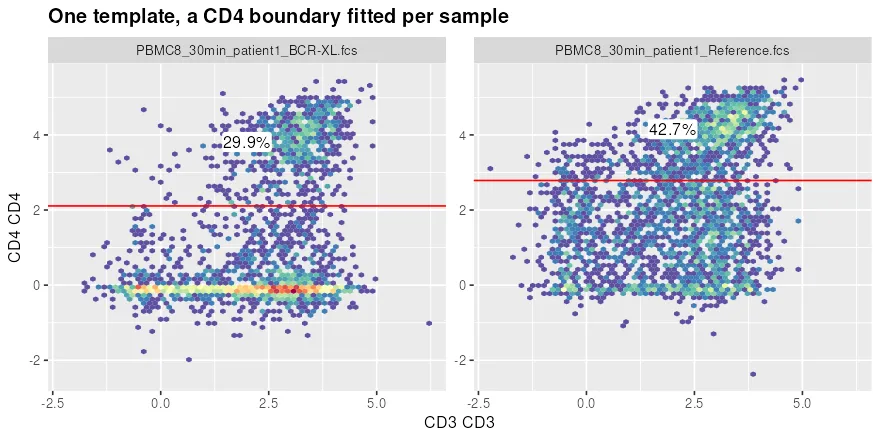

A fixed threshold would have reported one of those two frequencies wrongly. Fitting the boundary per sample is the difference between a number that describes the sample and a number that describes the gate.

What this does not solve

A template still encodes decisions. Someone chose CD45 as the first gate, chose mindensity over flowClust, chose min=2 rather than 1.5, and chose to measure CD4 within CD3. Those choices are written down and reviewable now, which is the gain, and they are still choices. Clustering drops the hierarchy and groups events by the whole marker profile, which is the route to a population like CD20 that a sequential gate handles badly.