XGBoost

XGBoost is one of the most successful algorithms for tabular data. It builds an ensemble of decision trees sequentially, each correcting the errors of the previous ones. This page walks a complete classification workflow from training to interpretation.

Every code block runs in a container in the companion repository, so the numbers and figures are real.

Train a basic model

import xgboost as xgb
from sklearn.datasets import make_classification
from sklearn.model_selection import train_test_split, cross_val_score, StratifiedKFold
from sklearn.metrics import classification_report, roc_auc_score

X, y = make_classification(n_samples=2000, n_features=20, n_informative=10,
                           n_redundant=3, weights=[0.7, 0.3], flip_y=0.05, random_state=42)
X_train, X_test, y_train, y_test = train_test_split(
    X, y, test_size=0.2, random_state=42, stratify=y)

model = xgb.XGBClassifier(n_estimators=100, max_depth=4, learning_rate=0.1,
                          random_state=42, eval_metric="logloss")
cv = StratifiedKFold(n_splits=5, shuffle=True, random_state=42)
print(cross_val_score(model, X_train, y_train, cv=cv, scoring="roc_auc").mean())

Cross-validated ROC-AUC: 0.9286 (+/- 0.0245)
Test ROC-AUC: 0.9477
              precision    recall  f1-score   support
    Negative       0.89      0.93      0.91       276
    Positive       0.84      0.75      0.79       124
    accuracy                           0.88       400

Key hyperparameters

Parameter	Default	Effect
n_estimators	100	Number of trees; more capacity, slower
max_depth	6	Tree depth; deeper is more complex
learning_rate	0.3	Step shrinkage; lower needs more trees, generalizes better
subsample	1.0	Fraction of rows per tree
colsample_bytree	1.0	Fraction of columns per tree
min_child_weight	1	Minimum leaf weight; higher is more conservative
reg_alpha / reg_lambda	0 / 1	L1 / L2 regularization

The most impactful to tune are learning_rate, max_depth, n_estimators, and subsample.

Hyperparameter tuning

RandomizedSearchCV searches the space efficiently.

from sklearn.model_selection import RandomizedSearchCV
from scipy.stats import randint, uniform

search = RandomizedSearchCV(
    xgb.XGBClassifier(random_state=42, eval_metric="logloss"),
    {"n_estimators": randint(100, 500), "max_depth": randint(3, 8),
     "learning_rate": uniform(0.01, 0.3), "subsample": uniform(0.6, 0.4),
     "colsample_bytree": uniform(0.6, 0.4), "min_child_weight": randint(1, 10),
     "reg_alpha": uniform(0, 1), "reg_lambda": uniform(0.5, 2)},
    n_iter=50, cv=cv, scoring="roc_auc", random_state=42, n_jobs=-1)
search.fit(X_train, y_train)
print(f"Best ROC-AUC: {search.best_score_:.4f}")

Best ROC-AUC: 0.9341
  colsample_bytree: 0.9906
  learning_rate: 0.1333
  max_depth: 7
  n_estimators: 484
  subsample: 0.7958
Tuned Test ROC-AUC: 0.9428

Tuning lifted the cross-validated ROC-AUC from 0.929 to 0.934. On this particular test split the tuned model scored about the same as the default; tuning improves the expected score, not every single split.

Early stopping

Instead of guessing n_estimators, train many and stop when validation stops improving.

model_es = xgb.XGBClassifier(n_estimators=1000, max_depth=4, learning_rate=0.05,
                             random_state=42, eval_metric="logloss",
                             early_stopping_rounds=20)
model_es.fit(X_train_es, y_train_es, eval_set=[(X_val, y_val)], verbose=False)
print(f"Best iteration: {model_es.best_iteration}")

Best iteration: 370
Best validation logloss: 0.2321

Set n_estimators high and let early_stopping_rounds=20 find the right number.

Feature importance

pd.DataFrame({"feature": feature_names,
             "importance": best_model.feature_importances_}).sort_values(
    "importance", ascending=False).head(6)

   feature  importance
feature_14    0.138053
feature_17    0.090913
feature_18    0.083418
feature_16    0.078228
 feature_9    0.068921
 feature_2    0.065309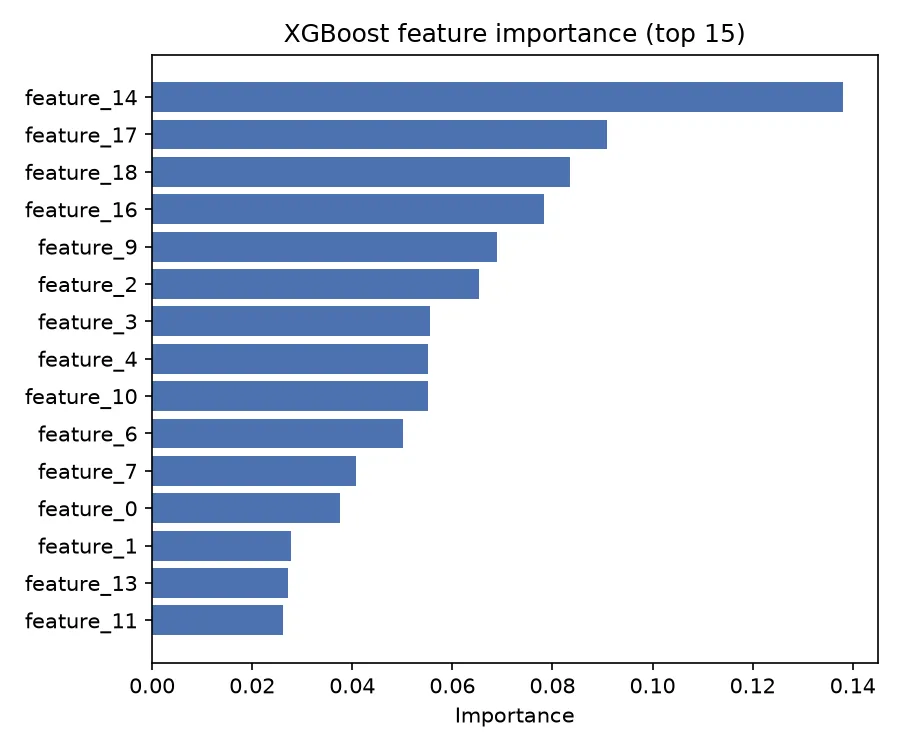

SHAP values

Feature importance says which features matter, not how they affect predictions. SHAP (SHapley Additive exPlanations) explains individual predictions.

import shap

explainer = shap.TreeExplainer(best_model)
shap_values = explainer.shap_values(X_test)
shap.summary_plot(shap_values, X_test, feature_names=feature_names)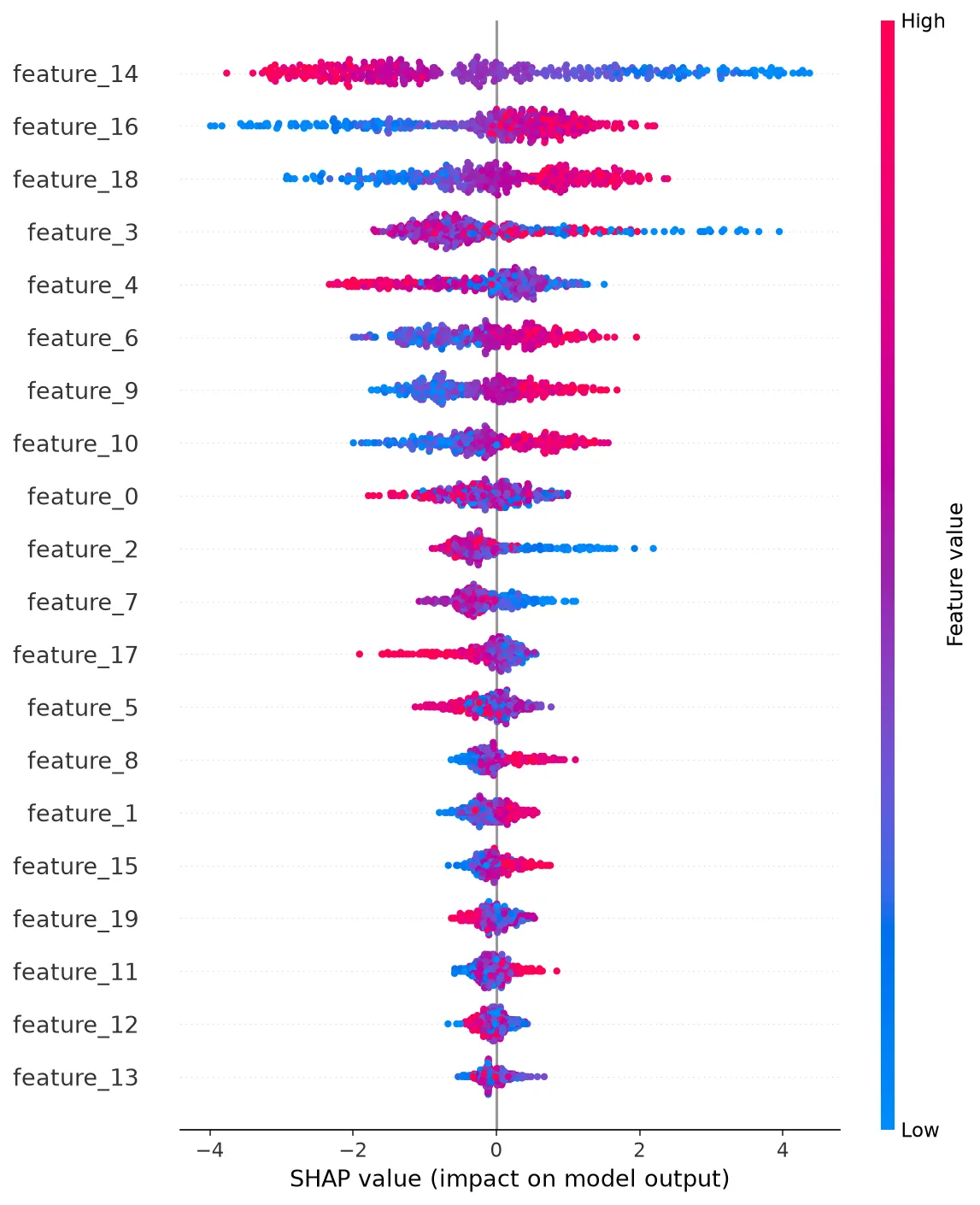

Each dot is one sample. The x-axis is the SHAP value (impact on the prediction); the color is the feature value (red high, blue low). For feature_14, high values push the prediction toward positive. Features are sorted by mean absolute SHAP value.

shap.summary_plot(shap_values, X_test, feature_names=feature_names, plot_type="bar")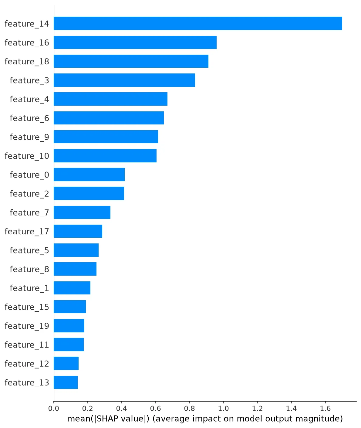

Summary

Step	What to do
Baseline	XGBClassifier(n_estimators=100, max_depth=4, learning_rate=0.1)
Tuning	RandomizedSearchCV with 50+ iterations
Early stopping	n_estimators=1000, early_stopping_rounds=20
Importance	model.feature_importances_ for a quick ranking
Interpretation	SHAP for per-sample explanations

Next steps

The next page covers LightGBM, which uses a different tree-building strategy that makes it faster on large datasets.