Linear & Logistic Regression

Linear and logistic regression are the foundation of supervised learning: fast, interpretable, and often surprisingly competitive. Understand them before moving to more complex models.

Every code block runs in a container in the companion repository, so the numbers are real.

Linear regression

Linear regression predicts a continuous target as a weighted sum of features.

from sklearn.datasets import make_regression
from sklearn.pipeline import Pipeline
from sklearn.preprocessing import StandardScaler
from sklearn.linear_model import LinearRegression
from sklearn.metrics import mean_squared_error, r2_score

X, y = make_regression(n_samples=500, n_features=10, n_informative=5,
                       noise=15, random_state=42)
X_train, X_test, y_train, y_test = train_test_split(X, y, test_size=0.2, random_state=42)

lr = Pipeline([("scaler", StandardScaler()), ("regressor", LinearRegression())])
lr.fit(X_train, y_train)
print(f"RMSE: {np.sqrt(mean_squared_error(y_test, lr.predict(X_test))):.2f}")
print(f"R2:   {r2_score(y_test, lr.predict(X_test)):.4f}")

RMSE: 16.21
R2:   0.9427

After scaling, coefficients show the relative importance and direction of each feature.

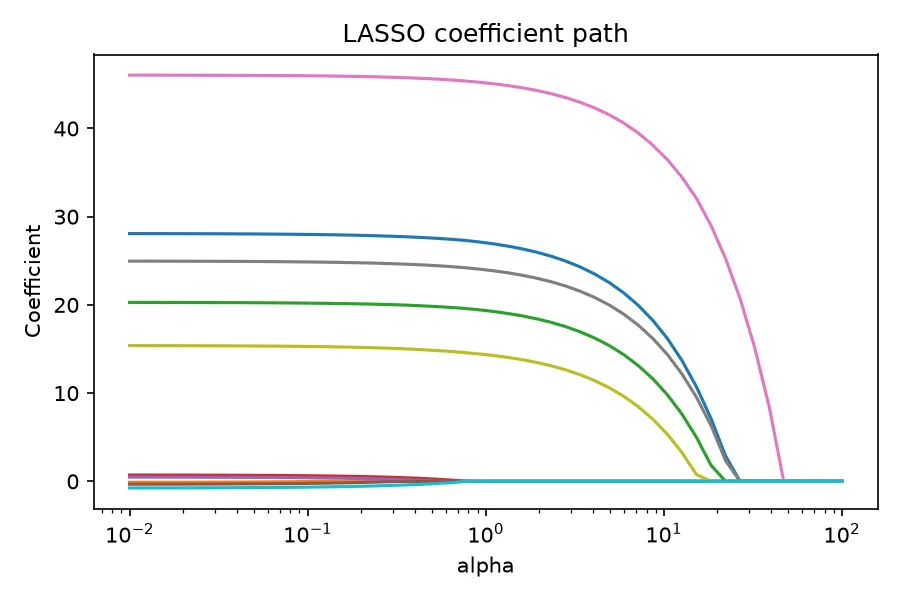
pd.DataFrame({"feature": feature_names,
             "coefficient": lr.named_steps["regressor"].coef_}).sort_values(
    "coefficient", key=abs, ascending=False)

  feature  coefficient
feature_6       46.052
feature_0       28.095
feature_7       24.972
feature_2       20.291
feature_8       15.396
feature_9       -0.757
feature_3        0.725
feature_4        0.488
feature_5       -0.335
feature_1       -0.123

The five informative features (6, 0, 7, 2, 8) have large coefficients; the rest sit near zero. The model recovered the signal.

Scale before interpreting

Coefficients are only comparable when features share a scale. Always StandardScaler before comparing them, or a feature in milligrams will dwarf one in kilograms even if they matter equally.

Regularization

Regularization penalizes large coefficients, reducing overfitting.

from sklearn.linear_model import Ridge, Lasso, ElasticNet
# fit Linear, Ridge(1), Ridge(10), Lasso(1), Lasso(10), ElasticNet(1, 0.5)

                       Model      RMSE       R2  Non-zero coefs
                      Linear 16.214131 0.942674              10
             Ridge (alpha=1) 16.206463 0.942728              10
            Ridge (alpha=10) 16.212423 0.942686              10
             LASSO (alpha=1) 16.470168 0.940850               5
            LASSO (alpha=10) 28.599540 0.821647               5
ElasticNet (alpha=1, l1=0.5) 27.512949 0.834942               9

• Ridge shrinks coefficients but keeps all 10 features; performance is unchanged.
• LASSO (alpha=1) zeros 5 features, keeping exactly the informative ones.
• LASSO (alpha=10) over-penalizes and hurts performance.
• Elastic Net blends both penalties.

The LASSO coefficient path shows how coefficients shrink to zero as regularization grows. Informative features survive longest.

Logistic regression

Logistic regression predicts class probability via a sigmoid of the weighted sum.

from sklearn.linear_model import LogisticRegression

X, y = make_classification(n_samples=1000, n_features=10, n_informative=5,
                           n_redundant=2, weights=[0.7, 0.3], random_state=42)
X_train, X_test, y_train, y_test = train_test_split(
    X, y, test_size=0.2, random_state=42, stratify=y)

log_reg = Pipeline([("scaler", StandardScaler()),
                    ("classifier", LogisticRegression(max_iter=1000, random_state=42))])
cv = StratifiedKFold(n_splits=5, shuffle=True, random_state=42)
print("CV ROC-AUC:", cross_val_score(log_reg, X_train, y_train, cv=cv, scoring="roc_auc").mean())

Cross-validated ROC-AUC: 0.8786 (+/- 0.0192)
Test ROC-AUC: 0.8595

Coefficients are log-odds; exponentiating gives odds ratios, which are easier to read.

lcoef = log_reg.named_steps["classifier"].coef_[0]
pd.DataFrame({"feature": feature_names, "coefficient": lcoef,
             "odds_ratio": np.exp(lcoef)}).sort_values("coefficient", key=abs, ascending=False)

  feature  coefficient  odds_ratio
feature_3       1.0415      2.8334
feature_5      -0.8766      0.4162
feature_0       0.8740      2.3964
feature_4      -0.8477      0.4284
feature_1      -0.3235      0.7236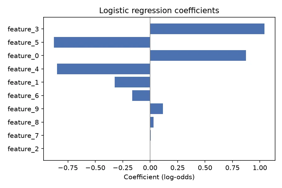

An odds ratio of 2.83 (feature_3) means a one-standard-deviation increase multiplies the odds of the positive class by 2.83. An odds ratio of 0.42 (feature_5) cuts them by 58%. Ratios near 1.0 have little effect.

The C parameter controls regularization (inverse of alpha). Performance is stable across a wide range, so the default C=1 is a fine start.

C=  0.01: ROC-AUC=0.8759
C=   0.1: ROC-AUC=0.8783
C=     1: ROC-AUC=0.8786
C=    10: ROC-AUC=0.8788
C=   100: ROC-AUC=0.8788

When to use it

Use linear or logistic regression when you need interpretable results, the relationship is roughly linear, or you want a fast baseline. Avoid it when the relationship is highly nonlinear or feature interactions matter and cannot be engineered by hand.

	Linear	Logistic
Task	Regression	Classification
Output	Continuous	Probability
Loss	Mean squared error	Log loss
Regularization	alpha (Ridge/LASSO)	C (inverse of alpha)
Interpretation	Coefficient = change in y per unit x	Odds ratio = multiplicative change in odds

Next steps

Linear models assume linearity. The next page covers XGBoost, which captures nonlinear patterns and interactions automatically.