End-to-End Pipeline

This page brings the section together into one workflow: load a dataset, compare four models with cross-validation, evaluate the best on a held-out test set, and inspect its feature importances.

Every code block runs in a container in the companion repository, so the numbers and figures are real.

1. Load and explore

X, y = make_classification(n_samples=3000, n_features=20, n_informative=10,
                           n_redundant=3, weights=[0.7, 0.3], flip_y=0.05, random_state=42)
print(f"Class distribution: {np.bincount(y)}")

Samples: 3000, Features: 20
Class distribution: [2081  919]
Class ratio: 30.63% positive

2. Split

X_train, X_test, y_train, y_test = train_test_split(
    X, y, test_size=0.2, random_state=42, stratify=y)

Hold the test set out until the very end. All model selection happens on the training set with cross-validation.

3. Compare models with cross-validation

models = {
    "Logistic Regression": Pipeline([("scaler", StandardScaler()),
                                     ("clf", LogisticRegression(max_iter=1000, random_state=42))]),
    "Random Forest": RandomForestClassifier(n_estimators=200, max_depth=10, random_state=42, n_jobs=-1),
    "XGBoost": xgb.XGBClassifier(n_estimators=200, max_depth=5, learning_rate=0.1,
                                 random_state=42, eval_metric="logloss"),
    "LightGBM": lgb.LGBMClassifier(n_estimators=200, num_leaves=31, learning_rate=0.1,
                                   random_state=42, verbose=-1),
}
cv = StratifiedKFold(n_splits=5, shuffle=True, random_state=42)
for name, model in models.items():
    s = cross_val_score(model, X_train, y_train, cv=cv, scoring="roc_auc")
    print(f"{name}: ROC-AUC = {s.mean():.4f} (+/- {s.std():.4f})")

Logistic Regression : ROC-AUC = 0.8893 (+/- 0.0171)
Random Forest       : ROC-AUC = 0.9444 (+/- 0.0114)
XGBoost             : ROC-AUC = 0.9466 (+/- 0.0121)
LightGBM            : ROC-AUC = 0.9488 (+/- 0.0117)

All three tree models beat logistic regression. LightGBM edges out the others, but the three tree models are within a standard deviation of each other.

4. Evaluate on the test set

for name, model in models.items():
    model.fit(X_train, y_train)
    print(name, roc_auc_score(y_test, model.predict_proba(X_test)[:, 1]))

LightGBM            Test ROC-AUC = 0.9341
Random Forest       Test ROC-AUC = 0.9307
XGBoost             Test ROC-AUC = 0.9286
Logistic Regression Test ROC-AUC = 0.9007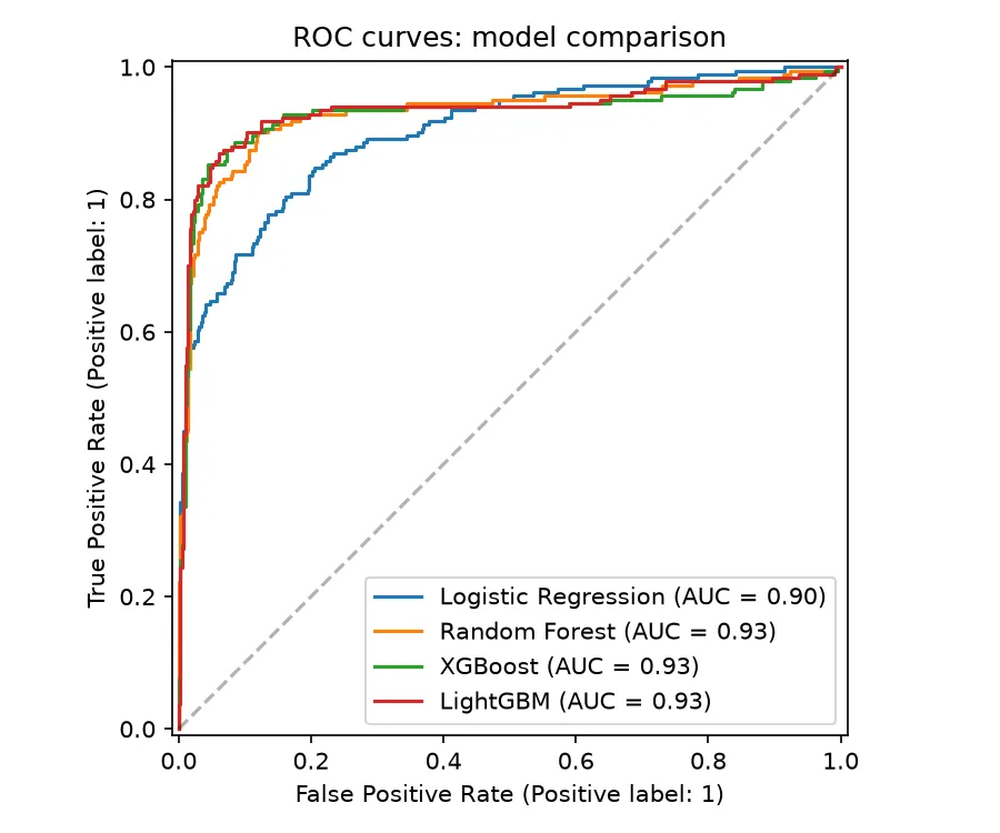

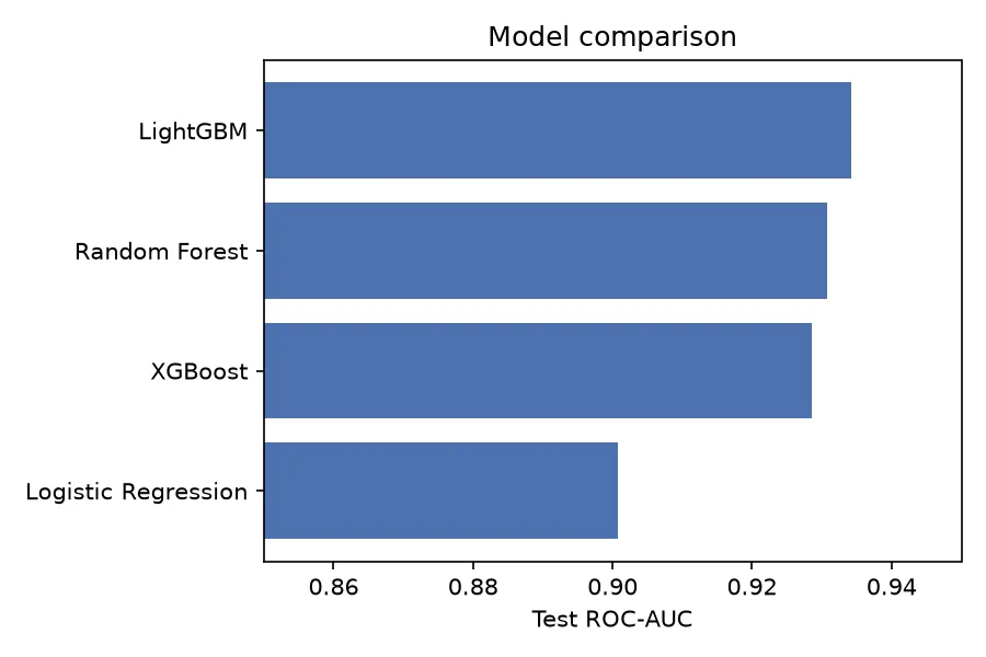
The three tree models cluster together; logistic regression sits lower, unable to capture the nonlinear structure.

5. Feature importance from the best model

best = models["LightGBM"]
pd.DataFrame({"feature": feature_names,
             "importance": best.feature_importances_}).sort_values(
    "importance", ascending=False).head(6)

   feature  importance
 feature_1         473
 feature_8         471
 feature_0         458
feature_17         414
feature_18         413
feature_10         399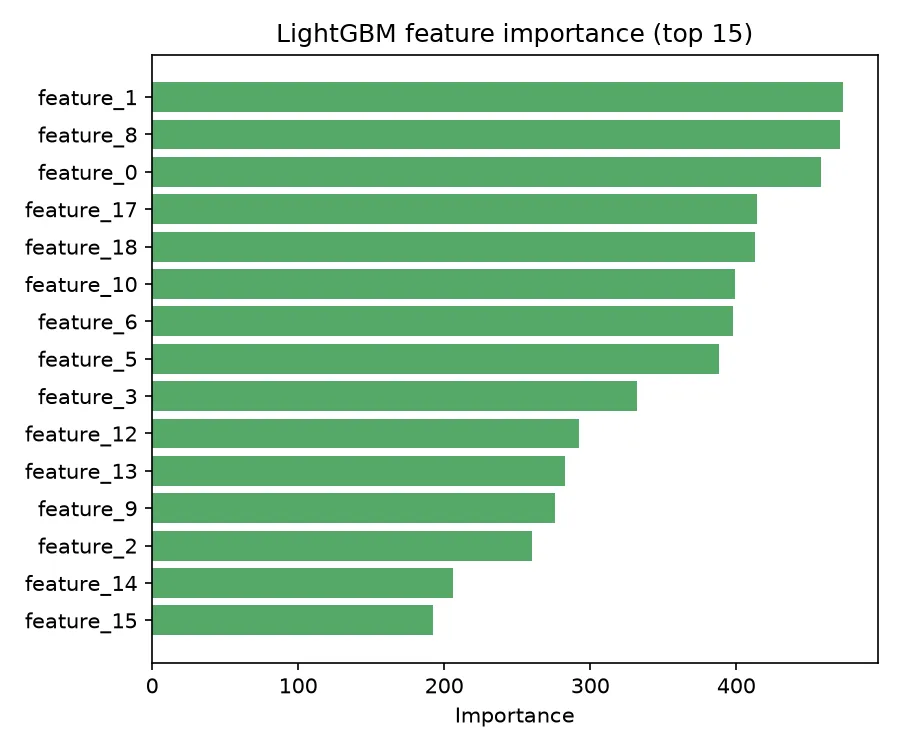

The complete checklist

1. Explore: shape, target balance, missing values, types.
2. Split: stratified train/test; hold the test out.
3. Preprocess: scale for linear models; tree models take raw features.
4. Compare: cross-validate several models on the training set.
5. Select: pick the best by cross-validated metric.
6. Tune: optionally with RandomizedSearchCV.
7. Evaluate: train on the full training set, score on the test set.
8. Interpret: feature importance and SHAP.

Do not peek at the test set

Keep the test set untouched until step 7. Using it during selection or tuning makes the performance estimate optimistic and unreliable.

When model differences are small

Here LightGBM, XGBoost, and Random Forest scored within half a percent. When models are this close, pick the one that is easiest to deploy, fastest to retrain, or most interpretable, or ensemble them. Do not over-optimize on the third decimal place.

Summary

Step	Tools
EDA	pandas, matplotlib
Preprocessing	StandardScaler, ColumnTransformer, Pipeline
Cross-validation	StratifiedKFold, cross_val_score
Tuning	RandomizedSearchCV, GridSearchCV
Evaluation	classification_report, roc_auc_score, RocCurveDisplay
Interpretation	feature_importances_, SHAP