Normalization

Load and filter

import numpy as np
import scanpy as sc
import matplotlib.pyplot as plt

sc.settings.verbosity = 3
np.random.seed(42)

adata = sc.read_10x_mtx("/opt/data/pbmc3k", var_names="gene_symbols",
                        make_unique=True)
adata.layers["counts"] = adata.X.copy()
adata.var["mt"] = adata.var_names.str.startswith("MT-")
sc.pp.calculate_qc_metrics(adata, qc_vars=["mt"], percent_top=None,
                           log1p=False, inplace=True)


def is_outlier(adata, metric, nmads):
    """Flag cells whose metric sits more than nmads MADs from the median.

    Args:
        adata: AnnData object holding the metric in .obs.
        metric: Column of adata.obs to test.
        nmads: Number of median absolute deviations for the cutoff.

    Returns:
        Boolean Series, True where the cell is an outlier.
    """
    values = adata.obs[metric]
    median = values.median()
    mad = (values - median).abs().median()
    return (values < median - nmads * mad) | (values > median + nmads * mad)


adata.obs["log1p_total_counts"] = np.log1p(adata.obs["total_counts"])
adata.obs["log1p_n_genes_by_counts"] = np.log1p(
    adata.obs["n_genes_by_counts"]
)
adata.obs["outlier"] = (
    is_outlier(adata, "log1p_total_counts", 5)
    | is_outlier(adata, "log1p_n_genes_by_counts", 5)
    | is_outlier(adata, "pct_counts_mt", 3)
)
adata = adata[~adata.obs["outlier"]].copy()
sc.pp.filter_genes(adata, min_cells=3)
print(adata.shape)

(2428, 13474)

The shifted logarithm

# The shifted logarithm is the default normalization in
# sc-best-practices: scale each cell to a common library size, then
# take the log of the scaled counts.
sc.pp.normalize_total(adata, target_sum=1e4)
sc.pp.log1p(adata)
adata.layers["normalized"] = adata.X.copy()

raw = adata.layers["counts"][:3, :4].toarray()
normalized = adata.layers["normalized"][:3, :4].toarray()
print("raw counts:\n", raw)
print("shifted log:\n", np.round(normalized, 3))

raw counts:
 [[0. 0. 0. 0.]
 [0. 0. 0. 0.]
 [0. 0. 0. 0.]]
shifted log:
 [[0. 0. 0. 0.]
 [0. 0. 0. 0.]
 [0. 0. 0. 0.]]

Analytic Pearson residuals

# The analytic Pearson residuals are the alternative sc-best-practices
# recommends. They model counts with an overdispersed Poisson and need
# no library-size scaling, and they are the basis of the Pearson
# flavour of highly variable gene selection.
adata_pearson = adata.copy()
adata_pearson.X = adata.layers["counts"].copy()
sc.experimental.pp.normalize_pearson_residuals(adata_pearson)

x_sample = adata_pearson.X[:3, :4]
if hasattr(x_sample, "toarray"):
    x_sample = x_sample.toarray()
print("pearson residuals:\n", np.round(x_sample, 3))

pearson residuals:
 [[-0.061 -0.035 -0.035 -0.035]
 [-0.07  -0.04  -0.04  -0.04 ]
 [-0.064 -0.037 -0.037 -0.037]]

Comparing the transforms

def gene_mean_variance(matrix):
    """Return per-gene mean and variance from a cells-by-genes matrix.

    Args:
        matrix: Cells-by-genes matrix, sparse or dense.

    Returns:
        Tuple of per-gene means and per-gene variances.
    """
    if hasattr(matrix, "toarray"):
        matrix = matrix.toarray()
    return matrix.mean(axis=0), matrix.var(axis=0)


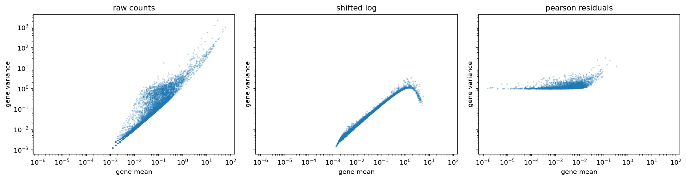
transformed = {
    "raw counts": adata.layers["counts"],
    "shifted log": adata.layers["normalized"],
    "pearson residuals": adata_pearson.X,
}

fig, axes = plt.subplots(1, 3, figsize=(15, 4), sharex=True, sharey=True)
for ax, (name, matrix) in zip(axes, transformed.items()):
    means, variances = gene_mean_variance(matrix)
    ax.scatter(means, variances, s=2, alpha=0.2)
    ax.set_xscale("log")
    ax.set_yscale("log")
    ax.set_title(name)
    ax.set_xlabel("gene mean")
    ax.set_ylabel("gene variance")
plt.tight_layout()
plt.savefig("outputs/normalization_meanvar.png", dpi=150,
            bbox_inches="tight")
plt.close()

Mean-variance scatter per gene for raw counts, the shifted logarithm and the Pearson residuals. Raw counts show variance rising steeply with the mean, the shifted logarithm compresses most genes onto a flat band, and the Pearson residuals sit closest to a mean-independent cloud.