MCIA: Multiple Co-Inertia Analysis

MCIA is the quick look you take before anything else. It finds a single low-dimensional space where all four layers are projected at once, chosen so that the layers agree as much as possible along each axis. No labels, no distributional assumptions, no model to train. It runs in seconds and tells you whether the layers share any structure worth integrating.

It is the multi-table generalization of co-inertia analysis. Where co-inertia relates two tables, MCIA relates all of them to one common reference, so every layer gets coordinates in the same space and you can see which layers pull together and which drift apart.

How it works

Each block is ordinated on its own, then a co-inertia step finds synthetic axes that maximize the covariance between the blocks’ projections. Two numbers come out. The pseudo-eigenvalue of each axis says how much shared co-structure that axis captures. The RV coefficient between two blocks, a multivariate correlation bounded between 0 and 1, says how much structure a pair of layers has in common. Because it works from cross-product matrices rather than a full decomposition, MCIA is fast and stable when the samples are few.

MCIA expects complete cases, so missing values are imputed to feature medians to keep all 200 patients. This page is R only: omicade4 has no mainstream Python implementation. It runs in the pinned multi-omics container, with the CLL data from the MOFAdata package inside it.

Running it

One call runs the analysis; the RV coefficients come from a short analytical helper.

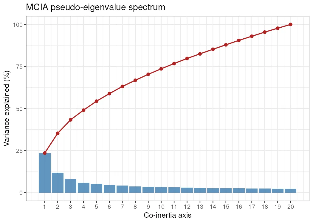
library(omicade4)
mcia_res <- mcia(data_list, cia.nf = 10)   # data_list: 4 data frames, features x 200
pe <- mcia_res$mcoa$pseudoeig              # per-axis shared inertia
sv <- mcia_res$mcoa$SynVar                 # global sample coordinates

The pseudo-eigenvalue spectrum drops fast. Axis 1 holds 23.5% of the shared inertia and Axis 2 another 11.7%, so the first two axes carry a third of the co-structure.

Plot the samples in the global space and color by IGHV. Axis 1 separates the two subtypes.

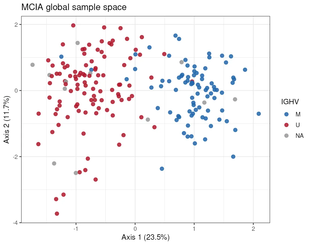
A Wilcoxon test on the Axis 1 scores confirms it at p = 3.3e-29. Every method in this section, factor-based, network-based, supervised, and now ordination-based, puts IGHV on its leading axis.

How much the layers share

The RV coefficients quantify the pairwise overlap MCIA is integrating.

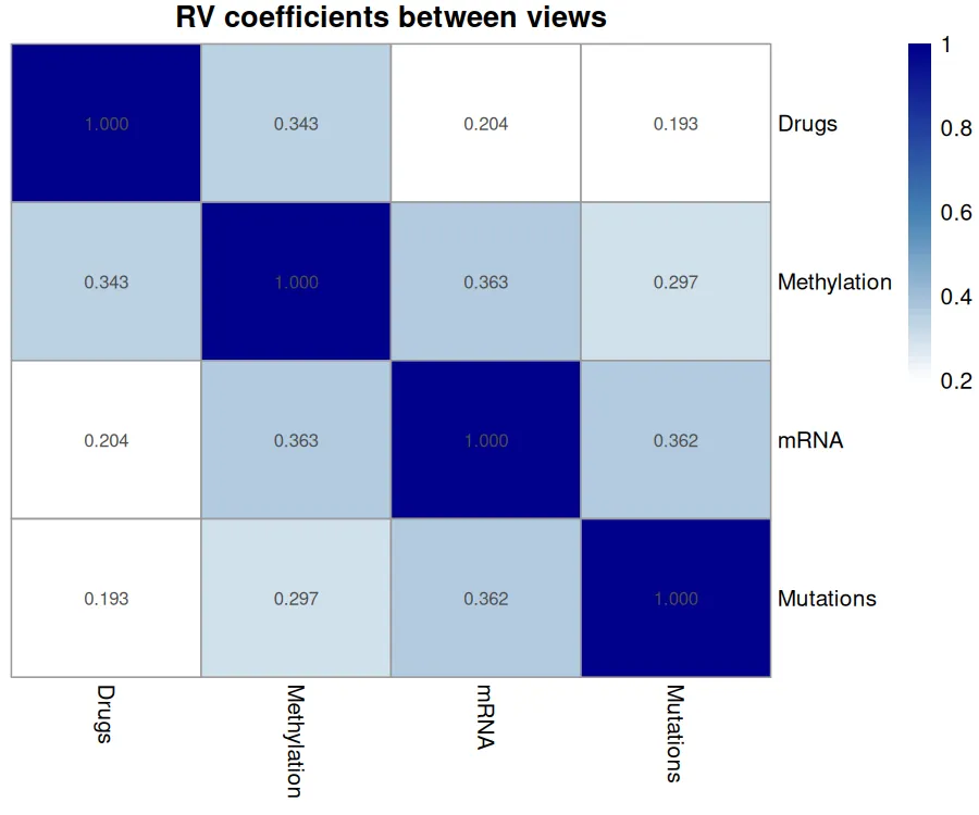
The values are moderate across the board, from 0.19 to 0.36. Methylation, mRNA, and mutations are the most connected trio, each pair near 0.36, while drug response shares the least with the molecular layers. That is a reasonable prior for the whole section: the molecular layers reinforce each other, and the functional drug readout adds a partly independent view.

Where MCIA stops

MCIA gives an ordination and feature loadings, not clusters and not a classifier. It does not handle missing data, so you impute first. Treat it as the fast exploratory pass: confirm the layers share structure and see the dominant axis, then bring in MOFA for interpretable factors, SNF for subtypes, or DIABLO for a supervised panel.

The runnable script and the container are in the companion code repo under guides/multi-omics/mcia/.