Flow Cytometry Overview

For each cell that passes the laser, a flow cytometer records the fluorescence intensity on every detector, plus a set of forward and side scatter signals. The instrument writes the result as an FCS file, a matrix of events by parameters. The analysis turns that matrix into cell populations, and the first step is to read the file into R.

Conventional, spectral, and mass

Three instrument families feed the same downstream analysis. Once the data are on the computer, the difference that matters is compensation.

Family	Markers	Detection	Compensation
Conventional flow	8 to 15	one detector per fluorophore	required, from single stains
Spectral flow	20 to 40+	full spectrum per fluorophore	required, unmixing matrix
Mass cytometry (CyTOF)	40 to 50	mass spectrometry, metal tags	none

Conventional and spectral flow both produce spillover, where one fluorophore’s signal leaks into another detector; mass cytometry tags its antibodies with rare metals and reads mass, so it has none to correct. The compensation page covers the spillover case. Transformation, gating and clustering work the same way on all three families.

The FCS file

An FCS file follows a binary standard, and FCS3.1 is the common version. The file has three parts: a header with byte offsets, a text segment of keyword-value pairs, and a data matrix of events by parameters. The keywords carry the metadata that make an analysis reproducible: the cytometer, the acquisition date, the fluorophore on each detector, and the spillover matrix. Without them the data matrix can still be read, but it cannot be interpreted.

Reading one file

flowCore is the base package for flow cytometry data in R. The example below finds an FCS file that ships inside the package, opens it, and prints what flowCore sees: the number of events, the number of parameters, and the keyword pairs that describe the run.

library(flowCore)

# flowCore ships small FCS files inside the package. List them.
extdata_dir <- system.file("extdata", package = "flowCore")
fcs_files <- list.files(extdata_dir, pattern = "0877408774", full.names = TRUE)
fcs_files

# Open the first one without transforming the raw intensities.
fcs_path <- fcs_files[1]
frame <- read.FCS(fcs_path, transformation = FALSE)

# Dimensions: rows are events, columns are parameters.
dim(exprs(frame))
colnames(frame)

# The text segment holds the instrument metadata.
keyword(frame, c("$FIL", "$DATE", "$CYT", "FCSversion"))

[1] "/usr/local/lib/R/site-library/flowCore/extdata/0877408774.B08"
[2] "/usr/local/lib/R/site-library/flowCore/extdata/0877408774.E07"
[3] "/usr/local/lib/R/site-library/flowCore/extdata/0877408774.F06"
[1] 10000     8
[1] "FSC-H" "SSC-H" "FL1-H" "FL2-H" "FL3-H" "FL1-A" "FL4-H" "Time"
$`$FIL`
[1] "0877408774.B08"

$`$DATE`
[1] "03-Feb-06"

$`$CYT`
[1] "FACSCalibur"

$FCSversion
[1] "2"

The transformation = FALSE argument is deliberate. By default flowCore log-transforms the data on read, and compensation needs the raw fluorescence intensities. The correction is applied on the linear scale, before any transform. The compensation page picks up from this object.

The first plot

Every cytometry analysis starts with forward scatter against side scatter, which is roughly size against granularity. It is where you find the cells, and where you find the debris and the dead events you do not want.

library(ggcyto)
library(ggplot2)

dir.create("outputs", showWarnings = FALSE, recursive = TRUE)

scatter_plot <- ggcyto(frame, aes(x = `FSC-H`, y = `SSC-H`)) +
  geom_hex(bins = 80) +
  labs(title = "Forward against side scatter, one FACSCalibur file")

ggsave("outputs/cyto-fsc-ssc.png", plot = scatter_plot,
       width = 6, height = 5, dpi = 110, bg = "white")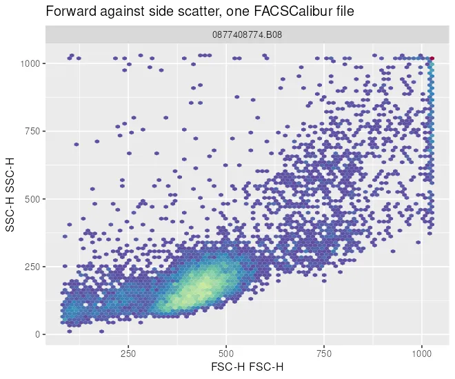

The vertical line at the right edge is the detector saturating. Forward scatter is stored in 1024 channels, and every event that exceeded the top of that range was recorded as 1023, so those events carry a bound rather than a value. A gate drawn through them is measuring the instrument.

What you keep

The keywords printed above are the minimum metadata for reproducing a gate: which file, which day, which instrument, and which standard. A real analysis adds a sample metadata table that maps each FCS file to a condition, a donor, and a panel. The FCS I/O page builds that table for a set of files.