Competing Risks & Fine-Gray

In real clinical data, events compete. A patient who dies of another cause can never relapse. Standard Kaplan-Meier treats that death as censoring and overstates the relapse risk. Competing-risks methods handle it correctly. This page estimates the cumulative incidence in R and Python, then fits the Fine-Gray model in R.

Every code block on this page runs in a container in the companion repository. The numbers and figures come from those real runs.

When to use competing-risks methods

Use them whenever more than one event type can end follow-up and they exclude each other: relapse versus death, or the specific cause of death versus other causes. Treating a competing event as ordinary censoring inflates the incidence of the event you care about.

The data

competing.csv has 200 patients. status is 0 for censored, 1 for relapse (the event of interest), and 2 for death without relapse. group is the treatment arm.

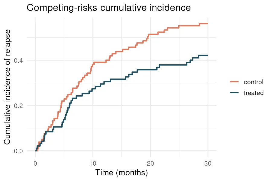
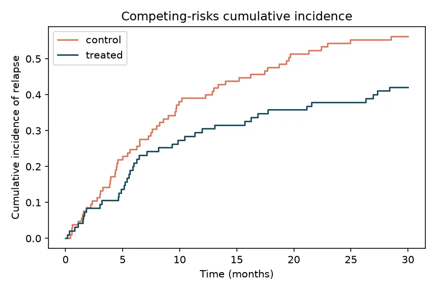
Cumulative incidence

The cumulative incidence function is the correct replacement for one-minus-Kaplan- Meier. It counts only the event of interest while letting competing events remove patients from the risk set. Both languages estimate it.

R
Python

library(tidycmprsk)

df$status <- factor(df$status, labels = c("censor", "relapse", "death"))
ci <- cuminc(Surv(time, status) ~ group, data = df)
ci

• Failure type "relapse"
strata    time   estimate   95% CI
control   30.0   0.562      0.460, 0.652
treated   30.0   0.421      0.320, 0.519

• Tests
outcome   statistic   df     p.value
relapse   3.88        1.00   0.049

from lifelines import AalenJohansenFitter

for grp in [0, 1]:
    m = df["group"] == grp
    ajf = AalenJohansenFitter()
    ajf.fit(df.loc[m, "time"], df.loc[m, "status"], event_of_interest=1)
    ajf.plot()

# Aalen-Johansen cumulative incidence, event_of_interest = 1 (relapse)
# control and treated curves, matching the R estimates above

By 30 months, 56% of controls have relapsed versus 42% of treated. Gray’s test, the competing-risks analogue of the log-rank test, gives p = 0.049. The plots agree.

R
Python

Cumulative incidence of relapse by arm (R)

The Fine-Gray model

To model covariate effects on the cumulative incidence directly, use the Fine-Gray subdistribution hazard model. It gives a subdistribution hazard ratio, the competing-risks counterpart of the Cox hazard ratio.

fg <- crr(Surv(time, status) ~ group, data = df)
tidy(fg, exponentiate = TRUE, conf.int = TRUE)

  term         estimate  conf.low  conf.high  p.value
  grouptreated    0.668     0.448      0.997    0.048

The subdistribution hazard ratio for treatment is 0.67, with a confidence interval just under 1 and p = 0.048. Treatment lowers the incidence of relapse, accounting for the competing risk of death.

Pitfalls and bioinformatics notes

Never use one-minus-Kaplan-Meier with competing risks. It ignores the competing event and overstates incidence. Use the cumulative incidence function.
Cause-specific and subdistribution hazards answer different questions. The cause-specific hazard (a Cox model on the event, censoring competitors) is for etiology. The Fine-Gray subdistribution hazard is for predicting incidence. Pick the one that matches your question.
Report absolute incidence, not just the hazard ratio. The cumulative incidence at a fixed time is what patients and clinicians actually weigh.
Tooling differs across languages. As here, some clinical methods are strong in R and absent in Python. Use the language that has the method.

Key points

Competing risks occur when one event prevents another. Kaplan-Meier mishandles them.
The cumulative incidence function is the correct estimate, and Gray’s test compares it across groups.
The Fine-Gray model gives subdistribution hazard ratios, and lives in R.
R and Python agree on the cumulative incidence; only R fits Fine-Gray.