Mixed-Effects & Repeated Measures

When you measure the same subjects more than once, the measurements are not independent. Two readings from one patient are more alike than readings from two patients. Ordinary regression ignores this and reports false confidence. Mixed-effects models add a random effect for the subject, so the clustering is handled honestly. This page models a longitudinal study, in R and Python.

Every code block on this page runs in a container in the companion repository. The numbers and figure come from those real runs.

When to use a mixed model

Use one whenever observations are grouped: repeated measures on the same subject, cells within a patient, samples within a batch, or patients within a hospital. The random effect captures the shared variation inside each group, which a plain regression would wrongly treat as independent evidence.

The data

longitudinal.csv has 20 subjects, each measured at 4 timepoints. The response falls over time, and each subject starts at its own baseline.

R

df <- read.csv("longitudinal.csv")
df$subject <- factor(df$subject)

Python

import pandas as pd

df = pd.read_csv("longitudinal.csv")

A spaghetti plot, one line per subject, shows the structure: each subject drifts downward from its own starting point.

R

library(ggplot2)

ggplot(df, aes(time, response, group = subject)) +
  geom_line(alpha = 0.4) +
  stat_summary(aes(group = 1), fun = mean, geom = "line", linewidth = 1.2)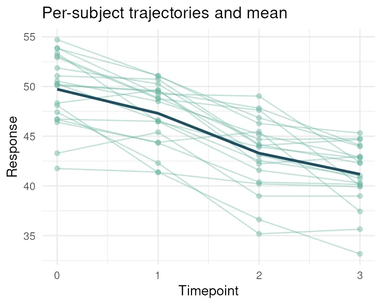

Python

for _, g in df.groupby("subject"):
    plt.plot(g["time"], g["response"], alpha=0.4, marker="o")
means = df.groupby("time")["response"].mean()
plt.plot(means.index, means.values, linewidth=2.5)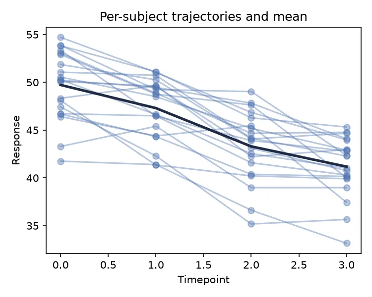

Fitting the mixed model

The model has a fixed effect for time, the trend we care about, and a random intercept for subject, which lets each subject have its own baseline.

R

library(lme4)
library(lmerTest)

fit <- lmer(response ~ time + (1 | subject), data = df)
summary(fit)

Random effects:
 Groups   Name        Variance Std.Dev.
 subject  (Intercept) 8.818    2.969
 Residual             2.897    1.702

Fixed effects:
            Estimate Std. Error      df t value Pr(>|t|)
(Intercept)  49.8206     0.7364 24.4002   67.65   <2e-16 ***
time         -2.9649     0.1702 59.0000  -17.42   <2e-16 ***

Python

import statsmodels.formula.api as smf

model = smf.mixedlm("response ~ time", df, groups=df["subject"]).fit()
model.summary()

            Coef.  Std.Err.    z    P>|z| [0.025 0.975]
Intercept   49.821    0.736  67.656 0.000 48.377 51.264
time        -2.965    0.170 -17.418 0.000 -3.299 -2.631
Group Var    8.817    2.091

Both fits agree. The response falls by 2.96 per timepoint, and that effect is highly significant. The random-intercept variance, 8.82, sits well above the residual variance, 2.90, which says subjects differ a lot at baseline. Ignoring that structure would have been a mistake.

Why not just ignore the subject?

Treating all 80 rows as independent is pseudoreplication. It pretends you have 80 independent measurements when you really have 20 subjects, each followed over time. That inflates the effective sample size, shrinks the standard errors, and hands you a p-value that is too small. The random intercept fixes this by crediting the evidence to subjects, not to individual rows.

Pitfalls and bioinformatics notes

• Match the random effect to the design. Repeated timepoints call for a random subject effect. Cells within patients call for a random patient effect. Get the grouping right.
• Random slopes, not just intercepts. If subjects change at different rates, add a random slope for time, written (time | subject) in lme4.
• This is the model behind many tools. limma’s duplicateCorrelation and several single-cell differential-expression methods are mixed models under the hood.
• You need enough groups. A handful of subjects gives an unstable variance estimate. Aim for more groups, not just more rows.

Key points

• Mixed models add random effects so clustered and repeated measures are analyzed honestly.
• The fixed effect is the trend of interest; the random effect captures group-level variation.
• Ignoring clustering is pseudoreplication and produces p-values that are too small.
• R and Python give matching fixed effects and variance components.

Further reading

• The lme4 documentation, and the statsmodels mixed linear models guide.
• The previous guides, Simple and Multiple regression, for the fixed-effects base.