ComBat and Its Limits

The second remedy rewrites the data instead of the model. ComBat, from the sva package, estimates for each batch and each gene a location shift and a scale change, shrinks those estimates across genes with an empirical Bayes prior, and subtracts the batch part. What is left is a matrix in which the batch is gone and the rest of the structure is kept, in principle.

The design route of the previous page is the default because it keeps the raw counts as the model input and keeps the batch in the error model. The removal route earns its place when the downstream method has no design formula to receive a batch term: a clustering, a heatmap, an integration of two studies, a plot that a reviewer wants to see without the batch in it. This page runs ComBat on the pasilla matrix, looks at what moved, and then measures the cost of the version that is tempting but wrong, correcting the counts and pretending they are raw.

ComBat on the transformed matrix

ComBat expects data on a roughly Gaussian scale, so it runs on the variance-stabilized matrix rather than the counts. The mod argument carries the condition, which tells ComBat what to protect while it removes the batch. Leaving mod out is a real mistake here: the library type and the condition are correlated in this design, so an unprotected ComBat would remove part of the knockdown signal along with the batch.

library(DESeq2)
library(pasilla)

# Counts and annotation, loaded the way the DESeq2 vignette does.
pas_anno <- system.file("extdata", "pasilla_sample_annotation.csv",
                        package = "pasilla", mustWork = TRUE)
coldata <- read.csv(pas_anno, row.names = 1)
coldata <- coldata[, c("condition", "type")]
rownames(coldata) <- sub("fb", "", rownames(coldata))
coldata$condition <- relevel(factor(coldata$condition), ref = "untreated")
coldata$type <- factor(coldata$type)

pas_cts <- system.file("extdata", "pasilla_gene_counts.tsv",
                       package = "pasilla", mustWork = TRUE)
cts <- as.matrix(read.csv(pas_cts, sep = "\t", row.names = "gene_id"))
cts <- cts[, rownames(coldata)]

# Keep genes with at least 10 reads total.
keep <- rowSums(cts) >= 10
cts <- cts[keep, ]

dds <- DESeqDataSetFromMatrix(cts, coldata, design = ~ condition)
vsd <- vst(dds, blind = TRUE)

# The PCA before correction, for the comparison.
pca_data <- plotPCA(vsd, intgroup = c("condition", "type"),
                    returnData = TRUE)

library(sva)

# Remove the library type, with the condition protected.
combat_mat <- ComBat(assay(vsd), batch = coldata$type,
                     mod = model.matrix(~ condition, coldata),
                     par.prior = TRUE)

Found 30 genes with uniform expression within a single batch (all zeros); these will not be adjusted for batch.

The message is part of the output worth reading. Thirty genes are all zeros within one batch, so ComBat has no information to adjust them with and leaves them alone. An adjustment method that reports what it cannot do is more trustworthy than one that adjusts silently.

The same PCA after correction

# The PCA of the corrected matrix, computed the same way.
vsd_combat <- vsd
assay(vsd_combat) <- combat_mat

pca_after <- plotPCA(vsd_combat, intgroup = c("condition", "type"),
                     returnData = TRUE)
pca_after[, c("PC1", "PC2", "condition", "type")]
attr(pca_after, "percentVar")

                  PC1         PC2 condition        type
treated1   -10.889226  0.97629296   treated single-read
treated2   -11.281014 -0.47683727   treated  paired-end
treated3   -10.978810 -0.37292181   treated  paired-end
untreated1   8.118550 -6.13952372 untreated single-read
untreated2   8.365270  2.56693483 untreated single-read
untreated3   8.559306  3.51822133 untreated  paired-end
untreated4   8.105924 -0.07216631 untreated  paired-end
[1] 0.83867422 0.07584055

# Correlation of PC2 with the library type, before and after.
type_code <- as.numeric(coldata$type == "paired-end")
round(c(before = cor(pca_data$PC2, type_code),
        after = cor(pca_after$PC2, type_code)), 3)

before  after
 -0.94   0.26

The second axis no longer separates the library types, and with it the structure of the matrix changes shape. PC1 now carries 84 percent of the variance, up from 56, because the batch that used to fill the second axis is gone, and PC2 is down from 30 percent to 8. The correlation of PC2 with the type indicator falls from -0.94 before the correction to 0.26 after, which is the removal working as advertised. The first axis still separates treated from untreated, which is the condition surviving. The next figure shows both panels side by side, on the same axes so the shrink of the second axis is visible.

library(ggplot2)

pca_data$panel <- "before"
pca_after$panel <- "after"
both_pca <- rbind(pca_data, pca_after)

combat_plot <- ggplot(both_pca, aes(PC1, PC2, color = condition,
                                    shape = type)) +
  geom_point(size = 3.5) +
  facet_wrap(~ panel) +
  scale_color_manual(values = c(untreated = "#2166ac", treated = "#b2182b")) +
  theme_minimal()

ggsave("outputs/combat-pca.png", combat_plot, width = 9, height = 4.5,
       dpi = 150, bg = "white")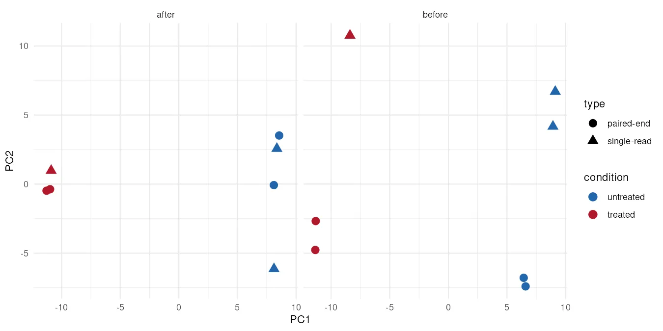

For a heatmap, a clustering, or a figure for a paper, this is the matrix to use. For a differential expression model it is not, and the reason is not a rule of thumb but a property of the method: ComBat returns point estimates with the batch removed and no accounting of the uncertainty that the removal added.

The tempting route, measured

The temptation is to correct the counts with ComBat_seq, the count-scale version of the method, and to run the differential model on the corrected matrix as if it were raw data. It is a real technique in the literature, so it deserves a measurement rather than a prohibition.

# ComBat_seq on the counts, protecting the condition.
adj_counts <- ComBat_seq(cts, batch = coldata$type,
                         group = coldata$condition)

# A differential run on the corrected counts, batch already removed.
dds_cseq <- DESeqDataSetFromMatrix(adj_counts, coldata,
                                   design = ~ condition)
dds_cseq <- DESeq(dds_cseq, quiet = TRUE)

res_cseq <- results(dds_cseq,
                    contrast = c("condition", "treated", "untreated"),
                    alpha = 0.05)
summary(res_cseq)

out of 9921 with nonzero total read count
adjusted p-value < 0.05
LFC > 0 (up)       : 755, 7.6%
LFC < 0 (down)     : 875, 8.8%
outliers [1]       : 1, 0.01%
low counts [2]     : 1347, 14%
(mean count < 5)
[1] see 'cooksCutoff' argument of ?results
[2] see 'independentFiltering' argument of ?results

# The design route from the previous page, for the comparison.
dds_batch <- DESeqDataSetFromMatrix(cts, coldata,
                                    design = ~ type + condition)
dds_batch <- DESeq(dds_batch, quiet = TRUE)

res_batch <- results(dds_batch,
                     contrast = c("condition", "treated", "untreated"),
                     alpha = 0.05)

sig_batch <- rownames(res_batch)[!is.na(res_batch$padj) &
                                 res_batch$padj < 0.05]
sig_cseq <- rownames(res_cseq)[!is.na(res_cseq$padj) &
                               res_cseq$padj < 0.05]

length(sig_batch)
length(sig_cseq)
length(intersect(sig_batch, sig_cseq))

[1] 1086
[1] 1630
[1] 1078

The corrected-counts run reports 1630 significant genes against the design route’s 1086, and it holds 1078 of the design route’s genes. It looks like power. It is optimism. The differential model treats the adjusted counts as observations and prices the batch removal at zero, so the standard errors are too small and the threshold too easy. The extra genes are not discoveries the design route missed. They are genes whose evidence got inflated by a method that the model cannot see.

Which route, when

The two routes have clean territories.

When the batch is recorded and every cell of the design table is occupied, the design term is the answer: it keeps the counts raw, it prices the nuisance variance honestly, and it is one word of code. When the downstream method has no design formula, or when the batch is the study itself in an integration, ComBat on transformed data is the standard tool, with the condition protected through mod.

When the batch is fully confounded with the condition, neither route can help, because the data never contained the information that separates them. That case is decided at the bench, on the day the samples are randomized.