Simple Linear Regression

Correlation says how strongly two variables move together. Regression goes further: it fits the line and gives you an equation. That equation predicts the outcome and puts a number, with a confidence interval, on the effect of the predictor. This page models cell viability as a function of gene expression, in R and Python.

Every code block on this page runs in a container in the companion repository. The numbers and figures come from those real runs.

When to use linear regression

Use it when you have a continuous outcome and want to model how it changes with a predictor. Unlike correlation, regression gives a slope in real units and lets you predict. It assumes the relationship is roughly linear and the residuals are roughly normal with constant spread.

The data

regression.csv has 50 samples with a predictor, expression, and a continuous outcome, viability.

R
Python

df <- read.csv("regression.csv")

import pandas as pd

df = pd.read_csv("regression.csv")

fit <- lm(viability ~ expression, data = df)
summary(fit)

Coefficients:
            Estimate Std. Error t value Pr(>|t|)
(Intercept)  87.1323     2.6373   33.04  < 2e-16 ***
expression   -4.5850     0.4061  -11.29 4.11e-15 ***

Residual standard error: 6.837 on 48 degrees of freedom
Multiple R-squared:  0.7265,  Adjusted R-squared:  0.7208
F-statistic: 127.5 on 1 and 48 DF,  p-value: 4.11e-15

import statsmodels.formula.api as smf

model = smf.ols("viability ~ expression", data=df).fit()
model.summary()

                 coef    std err          t      P>|t|      [0.025      0.975]
Intercept     87.1323      2.637     33.038      0.000      81.830      92.435
expression    -4.5850      0.406    -11.290      0.000      -5.401      -3.768
R-squared: 0.726

The two fits are identical to the decimal.

Reading the coefficients

Intercept, 87.1. The predicted viability when expression is zero. Here it is an extrapolation, since no sample has expression near zero, so read it with care.
Slope, -4.59. Each one-unit rise in expression lowers viability by about 4.6 percentage points. The 95% confidence interval runs from -5.40 to -3.77, so the effect is clearly negative.
p-value, 4e-15. The slope is very unlikely to be zero. There is a real relationship.
R-squared, 0.73. Expression explains about 73% of the variation in viability.

The fitted line and its confidence band:

R
Python

library(ggpubr)  # ggscatter builds the plot; stat_cor adds R and the p-value

ggscatter(df, x = "expression", y = "viability", add = "reg.line", conf.int = TRUE) +
  stat_cor(method = "pearson", p.accuracy = 0.001, r.accuracy = 0.01)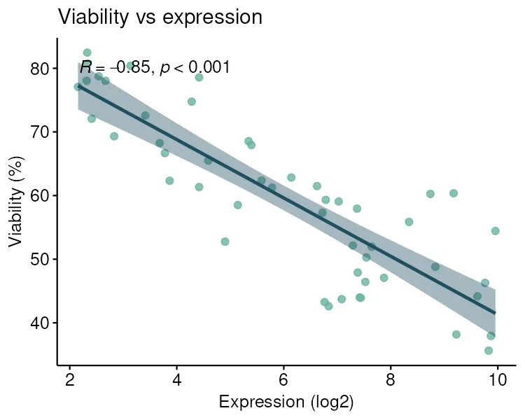

Viability against expression with the fitted line (R)

import numpy as np
import seaborn as sns

ax = sns.regplot(data=df, x="expression", y="viability")
r = np.sign(model.params["expression"]) * np.sqrt(model.rsquared)
ax.text(0.05, 0.1, f"R = {r:.2f}, p < 0.001", transform=ax.transAxes, va="bottom")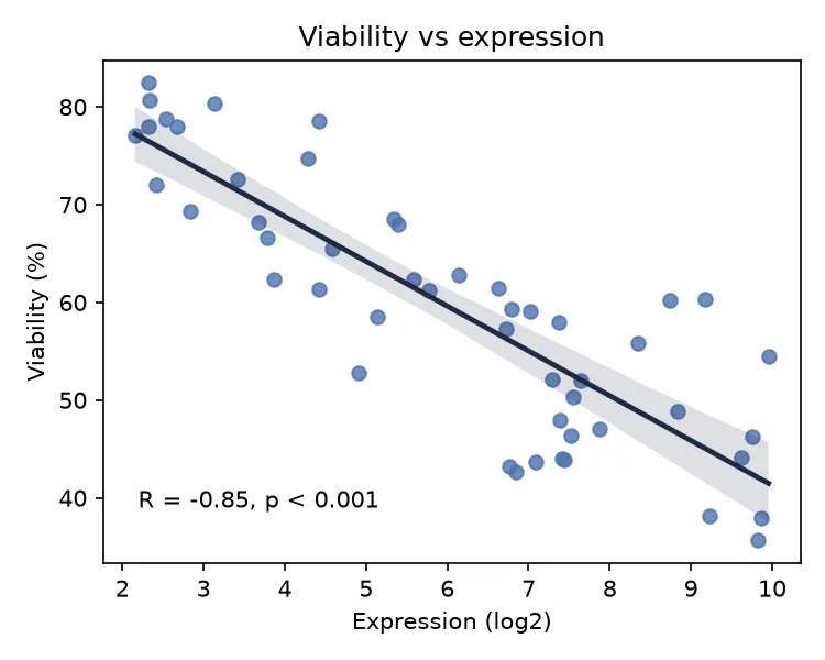

Viability against expression with the fitted line (Python)

Checking the fit

A model is only trustworthy if its residuals behave. The residuals-versus-fitted plot is the key diagnostic. You want a shapeless cloud around zero. A curve means the relationship is not linear. A funnel means the spread is not constant.

R
Python

diag <- data.frame(fitted = fitted(fit), resid = resid(fit))
ggscatter(diag, x = "fitted", y = "resid") +
  geom_hline(yintercept = 0, linetype = "dashed")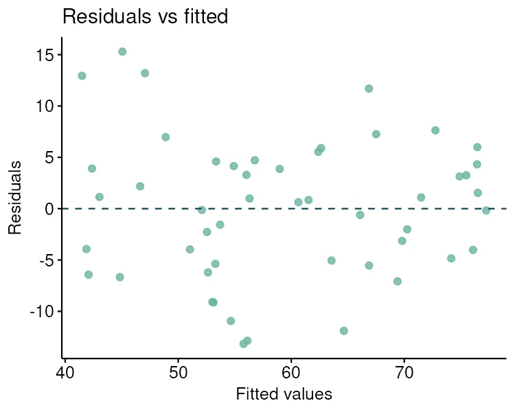

Residuals versus fitted values (R)

plt.scatter(model.fittedvalues, model.resid)
plt.axhline(0, ls="--")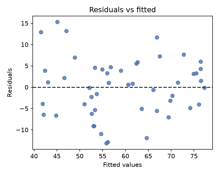

Residuals versus fitted values (Python)

The residuals scatter evenly around zero with no curve and no funnel. The linear model is a good fit here.

Pitfalls and bioinformatics notes

Do not extrapolate. The line is only trustworthy across the range of the data. The intercept here is an extrapolation.
Check the residuals, not just R-squared. A high R-squared with a curved residual plot still means the wrong model.
Outliers can dominate. A single high-leverage point can swing the slope. The residual plot helps you spot it.
Association, not cause. A significant slope does not prove that expression drives viability. A confounder can produce the same line.

Key points

Regression fits a line and gives a slope in real units, with a confidence interval.
The slope is the effect per unit of predictor; R-squared is the variance explained.
Always check the residuals-versus-fitted plot before trusting the model.
R and Python give identical fits.