Multiple Regression & Diagnostics

Real outcomes depend on more than one thing. Multiple regression adds predictors to the model, and its real power is adjustment: it estimates the effect of one variable while holding the others fixed. That is how you separate a genuine effect from a confounder. This page shows a confounded effect and how adjustment fixes it, in R and Python.

Every code block on this page runs in a container in the companion repository. The numbers and figure come from those real runs.

When to use multiple regression

Use it when several variables may influence the outcome, and especially when a predictor of interest is tangled up with others. Adjusting for the others gives the effect of your predictor that is not explained by them.

The data

multi_regression.csv has 80 samples with expression, age, and the outcome viability. In this dataset expression rises with age, and both lower viability. Age is a confounder.

R

df <- read.csv("multi_regression.csv")

Python

import pandas as pd

df = pd.read_csv("multi_regression.csv")

The confounded simple model

First fit viability on expression alone, ignoring age.

R

simple <- lm(viability ~ expression, data = df)
coef(simple)["expression"]

Simple model, expression coefficient: -5.595

Python

import statsmodels.formula.api as smf

simple = smf.ols("viability ~ expression", data=df).fit()
simple.params["expression"]

Simple model, expression coefficient: -5.595

Expression looks strongly harmful: each unit costs 5.6 points of viability. But some of that is really age, because older samples have higher expression and lower viability. The simple model blames expression for age’s effect.

The adjusted model

Now add age and let the model separate the two.

R

full <- lm(viability ~ expression + age, data = df)
summary(full)

             Estimate Std. Error t value Pr(>|t|)
(Intercept) 100.85572    2.74571  36.732  < 2e-16 ***
expression   -2.24678    0.66464  -3.380  0.00114 **
age          -0.53486    0.06541  -8.176 4.65e-12 ***

Multiple R-squared:  0.7016,  Adjusted R-squared:  0.6939

Python

full = smf.ols("viability ~ expression + age", data=df).fit()
full.summary()

                 coef    std err          t      P>|t|
Intercept    100.8557      2.746     36.732      0.000
expression    -2.2468      0.665     -3.380      0.001
age           -0.5349      0.065     -8.176      0.000
Adjusted R-squared: 0.694

Adjusted for age, the expression effect drops from -5.6 to -2.25. That is its real effect, holding age constant. Age itself costs about 0.53 points per year. Both fits agree to the decimal.

Seeing the adjustment

Plotting the expression coefficient before and after adjustment makes the confounding visible. The estimate moves sharply toward zero once age is in the model.

R

# expression coefficient and CI from each model, then plot with geom_errorbar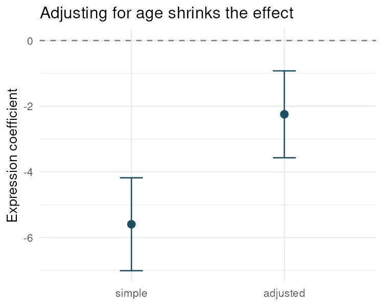

Python

# expression coefficient and CI from each model, then plot with errorbar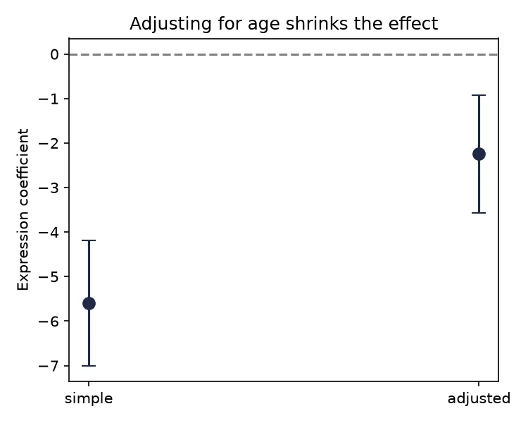

Pitfalls and bioinformatics notes

• “Holding others constant” is the whole point. Each coefficient is the effect of its variable with the others fixed. That is what makes adjustment work.
• Collinearity inflates uncertainty. When predictors are strongly correlated, the model cannot separate them and standard errors balloon. Check correlations first.
• Use adjusted R-squared. Plain R-squared always rises when you add predictors. Adjusted R-squared penalizes useless ones.
• Do not adjust for a mediator. Adjusting for a variable on the causal path between predictor and outcome hides the very effect you want. Confounder, yes; mediator, no.

Key points

• Multiple regression estimates each predictor’s effect while holding the others fixed.
• Adjusting for a confounder can change an effect substantially, as here from -5.6 to -2.25.
• Use adjusted R-squared, watch for collinearity, and do not adjust for mediators.

Further reading

• STHDA, multiple linear regression.
• An Introduction to Statistical Learning, chapter 3.
• The next guide, Logistic regression, for a binary outcome.