Checking Assumptions

Parametric tests like the t-test and ANOVA assume your data has a certain shape. Two assumptions matter most: the values are roughly normal, and the groups you compare have similar variance. This page shows how to check both, in R and Python. When a check fails, the last section shows what to do instead.

Every code block on this page runs in a container in the companion repository. The numbers and figures come from those real runs.

When to check assumptions

Check before you run a parametric test, not after. A t-test on skewed data, or an ANOVA on groups with very different variance, can give a p-value that looks fine but does not mean what you think. The checks take seconds and tell you whether the test you planned is the right one.

The data

assumptions_data.csv has 60 samples in two groups. The expression column is a roughly normal measurement. The intensity column is right-skewed, the way raw signal intensities often are. We will see one pass the normality check and one fail it.

R

df <- read.csv("assumptions_data.csv")

Python

import pandas as pd

df = pd.read_csv("assumptions_data.csv")

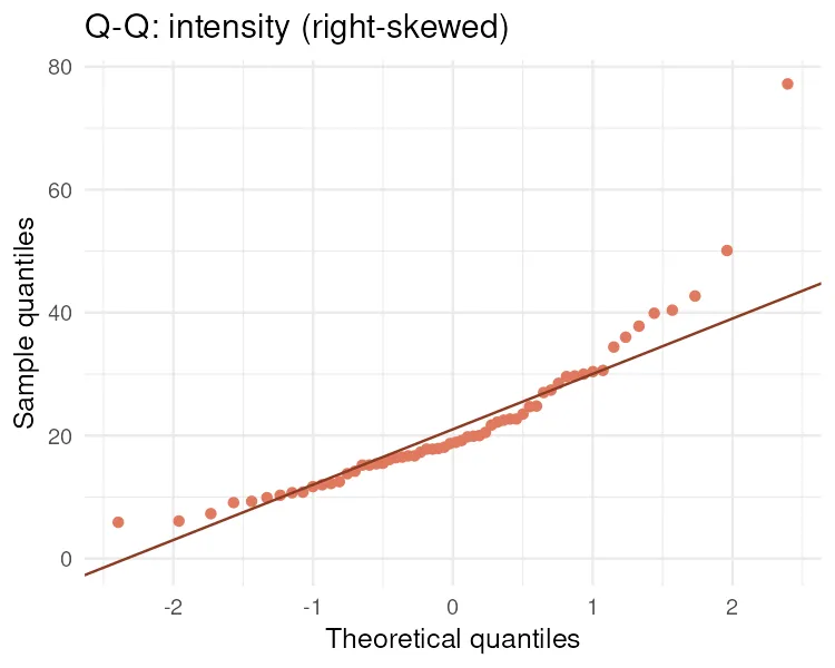
Testing normality

The Shapiro-Wilk test asks whether a sample could have come from a normal distribution. A large p-value means the data is consistent with normal. A small p-value means it is not. The visual companion is the Q-Q plot: normal data hugs the diagonal line.

R

shapiro.test(df$expression)
shapiro.test(df$intensity)

Shapiro-Wilk normality test
data:  df$expression
W = 0.99283, p-value = 0.9788

Shapiro-Wilk normality test
data:  df$intensity
W = 0.84679, p-value = 2.453e-06

Python

from scipy import stats

stats.shapiro(df["expression"])
stats.shapiro(df["intensity"])

Shapiro expression: W = 0.993, p = 9.788e-01
Shapiro intensity:  W = 0.847, p = 2.453e-06

Expression has a p-value of 0.98, far above 0.05, so it is consistent with a normal distribution. Intensity has a p-value of 0.000002, far below 0.05, so it is not normal. The Q-Q plots show the same story.

R

library(ggplot2)

ggplot(df, aes(sample = expression)) + stat_qq() + stat_qq_line()
ggplot(df, aes(sample = intensity)) + stat_qq() + stat_qq_line()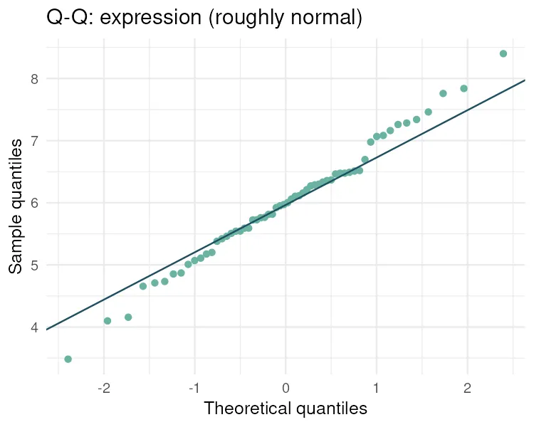

Python

from scipy import stats

stats.probplot(df["expression"], dist="norm", plot=plt)
stats.probplot(df["intensity"], dist="norm", plot=plt)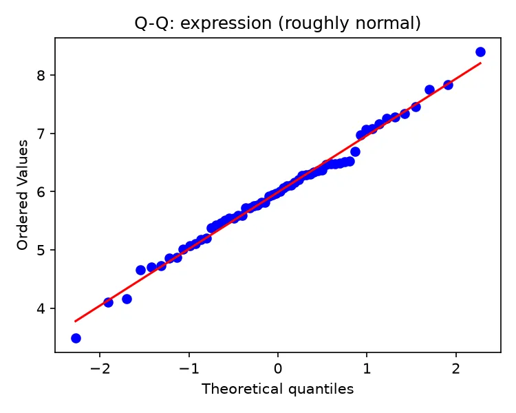

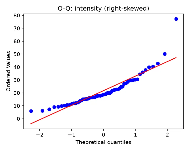
Expression sits on the line. Intensity bends away at both ends, the signature of a right-skewed variable.

Testing equal variance

Many tests, including the classic ANOVA, assume the groups being compared have similar variance. Levene’s test is the robust default. Bartlett’s test is more sensitive but assumes normality itself. A large p-value means the variances are similar.

R

library(car)

leveneTest(expression ~ factor(group), data = df)
bartlett.test(expression ~ group, data = df)

Levene's Test for Homogeneity of Variance (center = median)
      Df F value Pr(>F)
group  1  0.3297  0.568

Bartlett test of homogeneity of variances
Bartlett's K-squared = 0.1881, df = 1, p-value = 0.6645

Python

a = df.loc[df["group"] == "A", "expression"]
b = df.loc[df["group"] == "B", "expression"]

stats.levene(a, b, center="median")
stats.bartlett(a, b)

Levene:   W = 0.330, p = 5.680e-01
Bartlett: T = 0.188, p = 6.645e-01

Both tests give p-values around 0.6, well above 0.05, so the two groups have similar variance. A standard t-test or ANOVA is safe on this variable.

When an assumption fails

A failed check is useful information, not a dead end. You have three good options:

• Transform the variable. A log transform often turns a right-skewed variable, like our intensity column, into a roughly normal one. This is why expression is usually analyzed on the log scale.
• Use a non-parametric test. The Wilcoxon and Kruskal-Wallis tests rank the data and make no normality assumption.
• Use a variance-robust test. Welch’s t-test does not assume equal variance and is a safe default for two groups.

Pitfalls and bioinformatics notes

• The null is “normal”. A small p-value rejects normality. Do not read a large p-value as proof of normality, only as a lack of evidence against it.
• Big samples flag tiny deviations. With thousands of points, Shapiro-Wilk rejects normality for harmless wiggles. Lean on the Q-Q plot, not just the p-value.
• Counts are never normal. Do not test read counts for normality. Model them as counts.
• Check variance per comparison. Equal variance is a property of the groups you compare, not of the whole dataset.

Key points

• Shapiro-Wilk and the Q-Q plot check normality. A large p-value and points on the line mean normal.
• Levene’s and Bartlett’s tests check equal variance. A large p-value means the groups match.
• When a check fails, transform the variable, switch to a non-parametric test, or use a variance-robust test.

Further reading

• STHDA, normality test and homogeneity of variance.
• The previous guide, Descriptive statistics, for the Q-Q plot in more detail.
• The next guide, Sample size and power, on designing a study before you collect data.