Transformation and QC

Fluorescence intensities span several orders of magnitude and are skewed, so a raw scatter plot is unreadable. The transform that displays them has to do two things at once: compress the high end and resolve the low end where the negative, autofluorescent population sits. Linear compensation is done first, on the raw scale, and then the transform is applied.

The logicle transform

Logicle is the standard transform for flow cytometry. It is a biexponential function with a parameter for the width of the linear region near zero, which keeps the negative population visible instead of piling it against the axis. flowCore estimates the parameters from the data with estimateLogicle().

library(flowCore)

extdata_dir <- system.file("extdata", package = "flowCore")
fcs_files <- list.files(extdata_dir, pattern = "0877408774", full.names = TRUE)
frame <- read.FCS(fcs_files[1], transformation = FALSE)

# Compensate first, on the linear scale, with the single-stain matrix
# flowCore ships for this panel (the file stores no spillover keyword).
comp_path <- file.path(extdata_dir, "compdata", "compmatrix")
lines <- readLines(comp_path)
lines <- lines[nzchar(lines)]
chan <- strsplit(lines[3], "\t")[[1]]
spill <- do.call(rbind, lapply(lines[4:length(lines)], function(l) {
  as.numeric(strsplit(l, "\t")[[1]])
}))
colnames(spill) <- chan
rownames(spill) <- chan
frame <- compensate(frame, spill)

# Logicle on the fluorescence channels only; scatter and time stay linear.
fl_channels <- grep("^FL[1-4]-H$", colnames(frame), value = TRUE)
trans <- estimateLogicle(frame, fl_channels)
transformed <- transform(frame, trans)

# The first rows on the transformed scale.
head(exprs(transformed)[, fl_channels], 3)

        FL1-H     FL2-H    FL3-H    FL4-H
[1,] 4.278606 0.1759088 3.775404 3.807613
[2,] 3.861550 3.9366491 3.706503 3.966899
[3,] 4.330798 3.7732600 3.558080 4.258221

The transformed values are now on a scale where a biaxial plot separates populations. The exact parameters depend on the dynamic range of each channel, which is why estimateLogicle reads them from the data rather than taking a fixed value.

Arcsinh as the alternative

The arcsinh transform is a coarser cousin of logicle. It takes a single cofactor per channel, and it is the default in mass cytometry, where asinh(value / 5) is common. It does not adapt the linear region to the data the way logicle does, so it is a poorer choice when a negative population sits close to zero on a fluorescence instrument.

# Arcsinh with a cofactor of 150, a common fluorescence default.
cofactor <- 150
asinh_trans <- arcsinhTransform(
  transformationId = "asinh",
  a = 0,
  b = 1 / cofactor,
  c = 0
)
asinh_list <- transformList(fl_channels, tfun = asinh_trans)
transformed_asinh <- transform(frame, asinh_list)
head(exprs(transformed_asinh)[, fl_channels], 3)

        FL1-H     FL2-H     FL3-H    FL4-H
[1,] 2.122255 -1.048036 1.2158249 1.239618
[2,] 1.250208  1.552875 1.1100056 1.521909
[3,] 2.238147  1.297993 0.9057681 2.101034

The choice between logicle and arcsinh is mostly a question of how much you want the transform to adapt. Logicle adapts; arcsinh is fixed and portable across studies, which is why it is preferred when you need to compare cytometry to mass cytometry.

Quality control with flowAI

A sample degrades over the minutes it spends on the instrument. The acquisition rate drops, the signal drifts, and a tail of low-quality events accumulates. flowAI finds the time windows where the acquisition is stable and removes the rest, using three checks: a flowRate check on the number of events per time slice, a flowQ check on the fluorescence stability, and a flowMargin check on the dynamic range.

library(flowAI)

# flowAI returns a cleaned frame. The report and FCS outputs are off so the
# example stays self-contained.
clean_frame <- flow_auto_qc(
  frame,
  html_report = FALSE,
  mini_report = FALSE,
  fcs_QC = FALSE
)
head(exprs(clean_frame), 3)

Quality control for the file: 0877408774
57.3% of anomalous cells detected in the flow rate check.
0% of anomalous cells detected in signal acquisition check.
0.02% of anomalous cells detected in the dynamic range check.
     FSC-H SSC-H    FL1-H    FL2-H      FL3-H FL1-A    FL4-H Time
[1,]   350   111 582.3079 112.6991 -32.824924    37 127.9264  161
[2,]   222    95 529.6396 285.2898   2.619772    22 152.0697  161
[3,]   699   514 469.1847 421.3200 231.861008    11 662.6246  161

flow_auto_qc prints the fraction of events each check flags and returns the cleaned frame. This bundled teaching file is small, so its flow rate is unstable and the check removes a large fraction. On a full-size sample the removed fraction is typically a few percent. A real sample that loses a large fraction has a problem upstream, a clog or a low event rate, and no transform will fix that.

The three scales, side by side

The three scales side by side are worth looking at before you assume the transformation is doing what the textbook says.

library(ggplot2)

dir.create("outputs", showWarnings = FALSE, recursive = TRUE)

#' Put one channel of a frame into a plain data frame for plotting.
#'
#' @param frame A `flowFrame`.
#' @param channel The channel to extract.
#' @param scale_name A label for the scale, used as a facet title.
#' @return A data frame with the channel values and the scale label.
ChannelValues <- function(frame, channel, scale_name) {
  data.frame(value = exprs(frame)[, channel], scale = scale_name)
}

scales <- rbind(
  ChannelValues(frame, "FL1-H", "linear"),
  ChannelValues(transformed, "FL1-H", "logicle"),
  ChannelValues(transformed_asinh, "FL1-H", "arcsinh")
)
scales$scale <- factor(scales$scale,
                       levels = c("linear", "logicle", "arcsinh"))

scale_plot <- ggplot(scales, aes(x = value)) +
  geom_density(fill = "steelblue", alpha = 0.5) +
  facet_wrap(~scale, scales = "free") +
  labs(title = "FL1-H on three scales", x = "FL1-H", y = "density")

ggsave("outputs/cyto-transform-scales.png", plot = scale_plot,
       width = 9, height = 3, dpi = 110, bg = "white")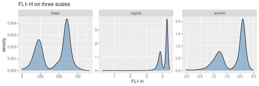

The two populations are already separated on the raw axis, and nothing was rescued here. That is a property of this file rather than of transformation. A FACSCalibur applies a logarithmic amplifier in hardware and stores the result as a channel number from 0 to 1023, so the values called linear above have already been through a log step.

The transformation still matters, and the reason is what a modern instrument does differently. A digital cytometer stores the raw photon count on a genuinely linear scale where a negative population, after compensation, sits in a spike at and below zero. On that data an untransformed plot really does collapse into the first bin, and logicle exists because a plain log cannot represent the negative values that compensation produces.

Between the two transformed panels, neither is more correct. Logicle fits its parameters from the data and arcsinh takes the cofactor you supply, so the shape of the low end is a choice in both cases.

The order, fixed

The order is compensation, QC, then transformation. Compensation is linear and must see the raw scale. QC removes events on the linear compensated scale, where the flowRate and flowMargin checks are meaningful. Transformation is nonlinear and is the last step before gating. Get the order wrong and the gates you draw downstream sit on the wrong coordinates. The automated gating page takes the cleaned, transformed object.