Model Evaluation

Choosing the right metric matters as much as choosing the right algorithm. A model that scores 85% accuracy can still miss most of the positive cases. This page covers the key metrics for classification and regression, when to use each, and how to read them.

Every code block runs in a container in the companion repository, so the numbers and figures are real.

The data and model

from sklearn.datasets import make_classification
from sklearn.model_selection import train_test_split
from sklearn.pipeline import Pipeline
from sklearn.preprocessing import StandardScaler
from sklearn.linear_model import LogisticRegression

X, y = make_classification(n_samples=1000, n_features=20, n_informative=5,
                           weights=[0.85, 0.15], random_state=42)
X_train, X_test, y_train, y_test = train_test_split(
    X, y, test_size=0.2, stratify=y, random_state=42)

pipeline = Pipeline([("scaler", StandardScaler()),
                     ("classifier", LogisticRegression(max_iter=1000, random_state=42))])
pipeline.fit(X_train, y_train)

Classification metrics

from sklearn.metrics import (accuracy_score, precision_score, recall_score,
                             f1_score, roc_auc_score, average_precision_score)

y_pred = pipeline.predict(X_test)
y_prob = pipeline.predict_proba(X_test)[:, 1]

print(f"Accuracy:  {accuracy_score(y_test, y_pred):.4f}")
print(f"Precision: {precision_score(y_test, y_pred):.4f}")
print(f"Recall:    {recall_score(y_test, y_pred):.4f}")
print(f"F1:        {f1_score(y_test, y_pred):.4f}")
print(f"ROC-AUC:   {roc_auc_score(y_test, y_prob):.4f}")
print(f"PR-AUC:    {average_precision_score(y_test, y_prob):.4f}")

Accuracy:  0.8450
Precision: 0.5000
Recall:    0.1935
F1:        0.2791
ROC-AUC:   0.8066
PR-AUC:    0.4368

The model looks fine at 84.5% accuracy. But recall is only 0.19: it finds fewer than one in five positive cases.

• Accuracy is the fraction of correct predictions. It is misleading with imbalanced data. A model that always predicts “negative” scores 85% here.
• Precision: of all samples predicted positive, how many are? High precision means few false positives.
• Recall (sensitivity): of all truly positive samples, how many did the model find? Recall of 0.19 means it misses 81% of the positives.
• F1 is the harmonic mean of precision and recall. Use it when both false positives and false negatives matter.
• ROC-AUC measures the ability to rank positives above negatives across all thresholds. It is threshold-independent.
• PR-AUC (average precision) focuses on the positive class and is more informative than ROC-AUC on imbalanced data.

Metric	Use when
Accuracy	Classes are balanced
Precision	False positives are costly (unnecessary treatments)
Recall	False negatives are costly (missed diagnoses)
F1	You need one number balancing precision and recall
ROC-AUC	Comparing models, threshold-independent
PR-AUC	Imbalanced data, the positive class is rare

Confusion matrix

from sklearn.metrics import confusion_matrix, ConfusionMatrixDisplay

cm = confusion_matrix(y_test, y_pred)
print(cm)
ConfusionMatrixDisplay(cm, display_labels=["Negative", "Positive"]).plot(cmap="Blues")

[[163   6]
 [ 25   6]]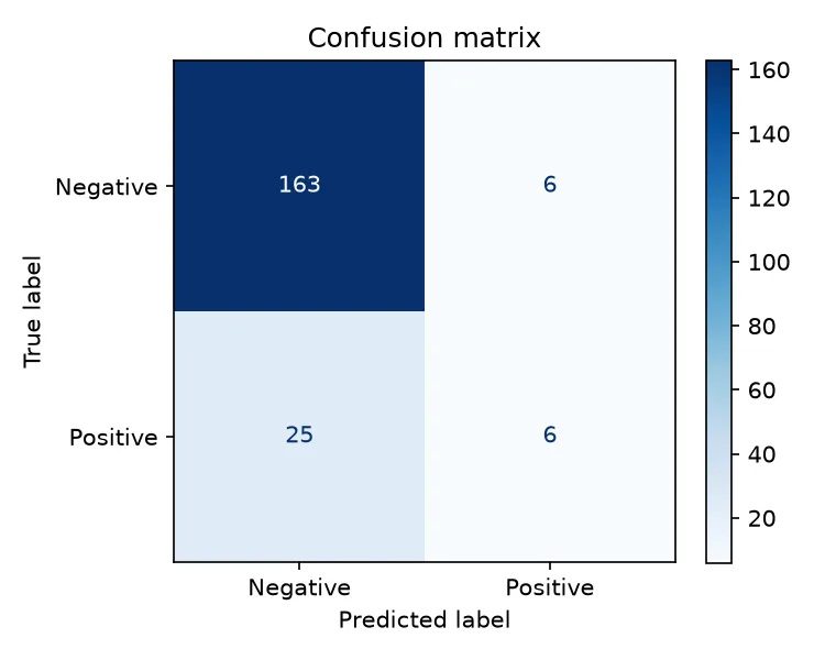

163 true negatives, 6 false positives, 25 false negatives, 6 true positives. The model is conservative: it predicts positive only when confident, so few false positives but many false negatives.

Classification report

from sklearn.metrics import classification_report

print(classification_report(y_test, y_pred, target_names=["Negative", "Positive"]))

              precision    recall  f1-score   support

    Negative       0.87      0.96      0.91       169
    Positive       0.50      0.19      0.28        31

    accuracy                           0.84       200
   macro avg       0.68      0.58      0.60       200
weighted avg       0.81      0.84      0.81       200

support is the number of samples per class. macro avg treats both classes equally; weighted avg accounts for class size.

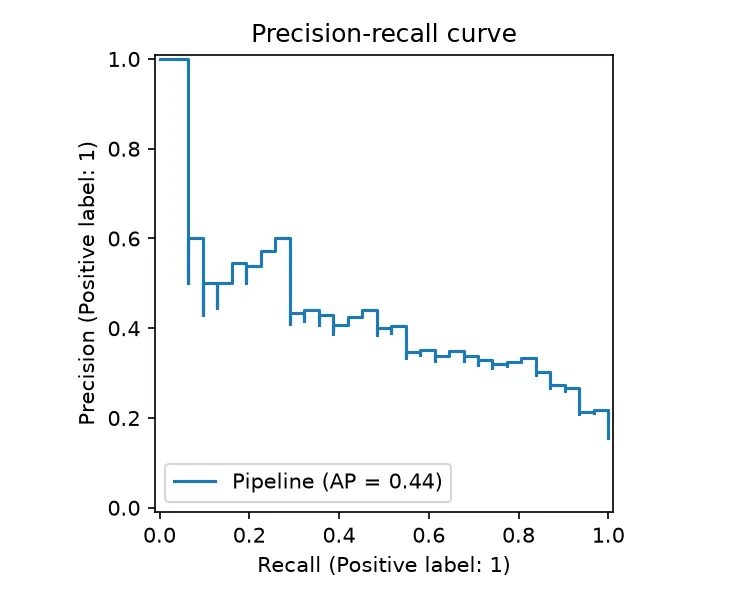
ROC and precision-recall curves

The ROC curve plots the true positive rate against the false positive rate at every threshold. For imbalanced data the precision-recall curve is more informative, because its baseline is the positive-class prevalence (about 0.15 here), not 0.5.

from sklearn.metrics import RocCurveDisplay, PrecisionRecallDisplay

RocCurveDisplay.from_estimator(pipeline, X_test, y_test)
PrecisionRecallDisplay.from_estimator(pipeline, X_test, y_test)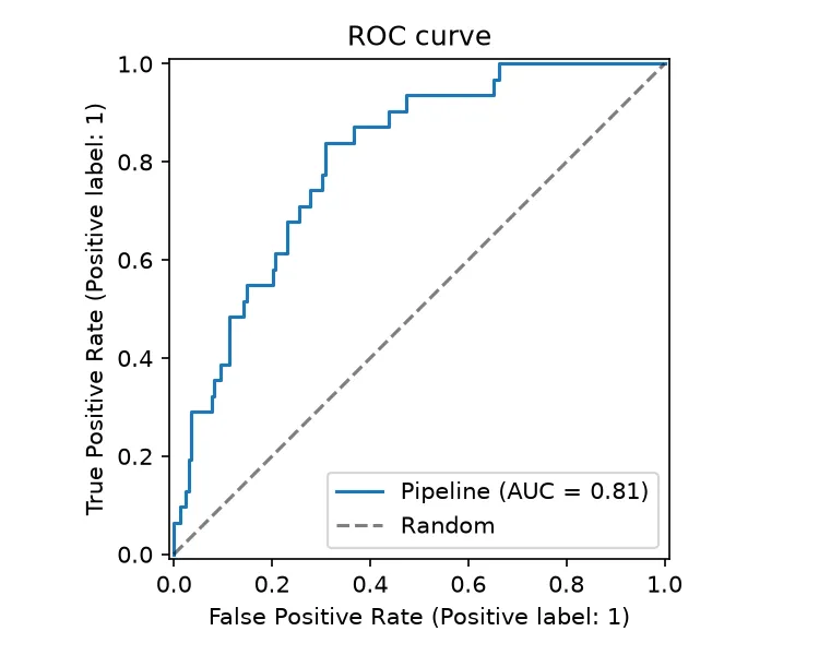

Adjusting the threshold

Classifiers use a default threshold of 0.5. Lowering it raises recall at the cost of precision.

for thr in (0.5, 0.3):
    y_thr = (y_prob >= thr).astype(int)
    print(f"Threshold {thr}: precision={precision_score(y_test, y_thr):.4f}, "
          f"recall={recall_score(y_test, y_thr):.4f}")

Threshold 0.5: precision=0.5000, recall=0.1935
Threshold 0.3: precision=0.4074, recall=0.3548

The right threshold depends on the cost of each error. In screening you want high recall and tolerate false positives; in target prioritization you want high precision.

Regression metrics

from sklearn.metrics import mean_squared_error, mean_absolute_error, r2_score

rmse = np.sqrt(mean_squared_error(y_test_r, y_pred_r))
print(f"RMSE: {rmse:.4f}")
print(f"MAE:  {mean_absolute_error(y_test_r, y_pred_r):.4f}")
print(f"R2:   {r2_score(y_test_r, y_pred_r):.4f}")

RMSE: 9.8539
MAE:  7.7979
R2:   0.9951

• RMSE is in target units and penalizes large errors most.
• MAE is in target units and treats all errors equally; it is more robust to outliers than RMSE.
• R-squared is the fraction of variance explained. 1.0 is perfect, 0.0 is a model that always predicts the mean.

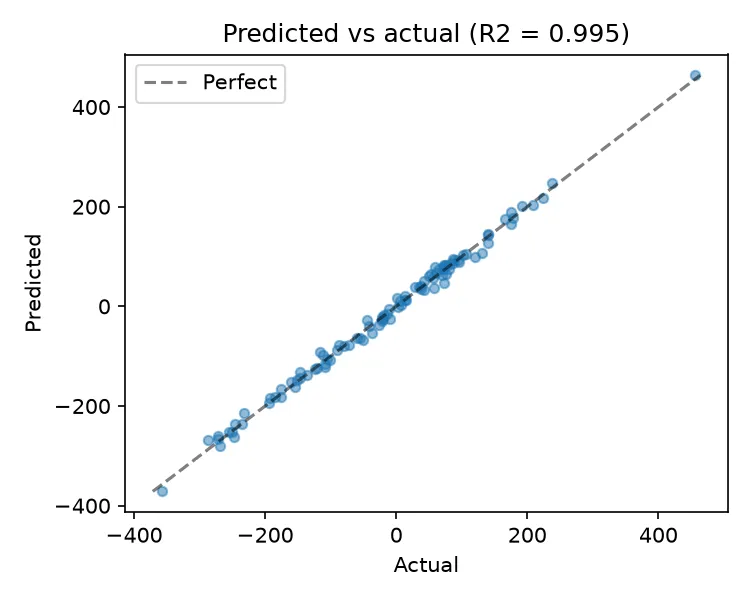
Points on the diagonal are perfect predictions. Systematic deviations mean the model is biased in some ranges.

Summary

Task	Primary metric	Secondary
Balanced classification	Accuracy, F1	ROC-AUC
Imbalanced classification	PR-AUC, F1	ROC-AUC, recall
Regression	RMSE	MAE, R-squared
Ranking	ROC-AUC	PR-AUC

Next steps

Now that you can evaluate models, the next page is an Algorithms Overview of the main tabular algorithms, with StatQuest videos explaining how each one works.