Gating

Gating is the classic answer to a cytometry file. You draw a boundary on a biaxial plot, keep the events inside it, and draw the next boundary on what is left. The chain of boundaries is the analysis, and the number a paper reports is the size of the population at the end of it.

In flowCore a gate is an object rather than an action. That matters more than it sounds, because an object can be printed, stored, passed to a function and compared with another one, while a boundary drawn with a mouse exists only inside the software that drew it.

A gate is an object

The example uses the first two samples of the Bodenmiller BCR-XL set, arcsinh transformed, with the channel names shortened to the bare marker so a gate can name the channel it cuts on.

library(flowCore)
library(HDCytoData)

fs <- Bodenmiller_BCR_XL_flowSet()[1:2]

# Arcsinh transform the surface markers, cofactor 5.
cd_channels <- grep("^CD", colnames(fs), value = TRUE)
asinh_trans <- arcsinhTransform(a = 0, b = 1 / 5, c = 0)
fs <- transform(fs, transformList(cd_channels, tfun = asinh_trans))

# The channel names carry the metal tag, CD45(In115)Dd. Shorten them to the
# marker so a gate and a plot can both name the channel.
colnames(fs) <- sub("\\(.*$", "", colnames(fs))

# A gate is an object. This one keeps everything above 2.0 on CD45.
cd45_gate <- rectangleGate(filterId = "CD45", "CD45" = c(2.0, Inf))
cd45_gate
class(cd45_gate)

Rectangular gate 'CD45' with dimensions:
  CD45: (2,Inf)
[1] "rectangleGate"
attr(,"package")
[1] "flowCore"

Applying it

Subset applies a gate and returns a smaller flowFrame. The count that comes out, and the count it came from, are the two numbers every gated result rests on.

frame <- fs[[1]]
cd45 <- Subset(frame, cd45_gate)

# Events before the gate, events after it, and the fraction kept.
nrow(exprs(frame))
nrow(exprs(cd45))
nrow(exprs(cd45)) / nrow(exprs(frame))

[1] 2838
[1] 2808
[1] 0.9894292

The hierarchy

A gate applies to the output of the gate above it. CD3 is measured within CD45, and CD4 within CD3, so the same CD4 boundary means something different depending on what came before it. That dependence is why a gating result is reported as a percentage of its parent and not only as a raw count.

cd3_gate <- rectangleGate(filterId = "CD3", "CD3" = c(2.0, Inf))
cd4_gate <- rectangleGate(filterId = "CD4", "CD4" = c(2.0, Inf))

#' Apply a chain of gates to one frame and count every population.
#'
#' @param frame A `flowFrame`.
#' @param gates A named list of gates, applied in the order given.
#' @return A data frame with one row per population, holding the event count and
#'   the percentage of the parent population. The root row has no parent.
GateChain <- function(frame, gates) {
  counts <- integer(0)
  parent <- frame
  for (name in names(gates)) {
    parent <- Subset(parent, gates[[name]])
    counts[name] <- nrow(exprs(parent))
  }
  all_counts <- as.integer(c(root = nrow(exprs(frame)), counts))
  parent_counts <- c(NA_integer_, utils::head(all_counts, -1))
  data.frame(
    population = c("root", names(counts)),
    count = all_counts,
    percent_of_parent = round(100 * all_counts / parent_counts, 1)
  )
}

chain <- list(CD45 = cd45_gate, CD3 = cd3_gate, CD4 = cd4_gate)

# The same three gates, applied to two different samples.
GateChain(fs[[1]], chain)
GateChain(fs[[2]], chain)

  population count percent_of_parent
1       root  2838                NA
2       CD45  2808              98.9
3        CD3  1843              65.6
4        CD4   648              35.2
  population count percent_of_parent
1       root  2739                NA
2       CD45  2697              98.5
3        CD3  1648              61.1
4        CD4   978              59.3

The two samples are the same patient at the same time point, one stimulated and one not. The same three boundaries call 35.2 percent of T cells CD4 positive in the first and 59.3 percent in the second. A difference that large is not a treatment effect on CD4, it is the boundary sitting in a different place relative to each sample’s distribution.

The gate, drawn

ggcyto puts the gate on the plot, which is the only way to see whether the boundary sits where the data separates.

library(ggcyto)
library(ggplot2)

dir.create("outputs", showWarnings = FALSE, recursive = TRUE)

gate_plot <- ggcyto(fs, aes(x = CD3, y = CD4)) +
  geom_hex(bins = 64) +
  geom_gate(cd4_gate) +
  labs(title = "One fixed CD4 boundary, two samples")

ggsave("outputs/cyto-manual-gate.png", plot = gate_plot,
       width = 8, height = 4, dpi = 110, bg = "white")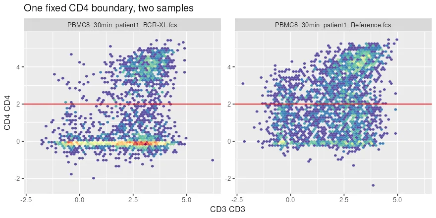

What a fixed boundary costs

The cut at 2.0 was a decision. Nothing in the data chose it, and the two samples do not have their CD4 populations in the same place, so one fixed boundary is right for at most one of them. Copying a gate across a plate is the normal way this is done, and it is the normal way a result drifts.

Two pages follow from that. Automated gating keeps the channel and the method fixed and lets each sample’s own distribution set the boundary. Harmonisation measures what the choice is worth, by moving one threshold and watching the reported frequency move with it.