SNF: Similarity Network Fusion

MOFA and MCIA work on features. SNF throws the features away and works on patients. It builds one patient-to-patient similarity network per layer, then fuses those networks into a single consensus network by letting strong edges in any one layer reinforce weak edges in the others. Clustering the fused network gives patient subtypes.

That shift, from a feature space to a similarity space, is what makes SNF non-linear and unusually robust when samples are few. It never has to decompose a 5000 by 200 matrix. It only needs the 200 by 200 table of how alike each pair of patients is.

How it works

Three steps. Build an affinity matrix per view from patient distances. Fuse the matrices with a message-passing update, where each network is nudged toward the others over several iterations until they agree. Cut the fused network into clusters with spectral clustering. The fusion is the clever part: a similarity that shows up in only one layer fades, while a similarity present across layers is amplified.

SNF expects complete cases, so missing values are imputed to feature medians to keep all 200 patients. This page is R only: SNFtool has no mainstream Python implementation. It runs in the pinned multi-omics container, and the CLL data comes from the MOFAdata package inside it.

Running it

Continuous views get a scaled Euclidean distance; the binary Mutations view gets a simple matching distance. The rest is three SNFtool calls.

library(SNFtool)
K <- 20; sigma <- 0.5

# One affinity matrix per view, then fuse, then cluster.
Wall  <- lapply(views, function(v) affinityMatrix(dist_of(v), K = K, sigma = sigma))
fused <- SNF(Wall, K = K, t = 20)
clusters <- spectralClustering(fused, K = 2)

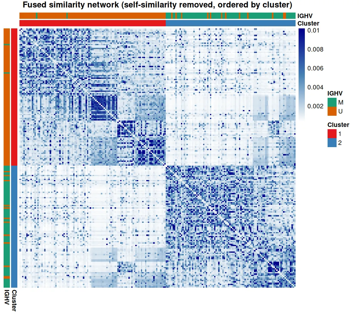
Ordered by cluster, the fused network shows two blocks of high within-group similarity, and the annotation bars line them up against IGHV status.

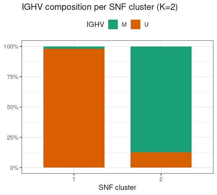
The two clusters are almost pure IGHV subtypes. Cluster 1 holds 104 unmutated patients against 2 mutated; cluster 2 holds 82 mutated against 12 unmutated. A Fisher exact test puts the association at p = 3.8e-40.

Which layer drives the fusion

Because SNF fuses networks rather than stacking features, you can ask which layer’s own clustering most agrees with the fused result. Cluster each view on its own, then measure the normalized mutual information against the fused clusters.

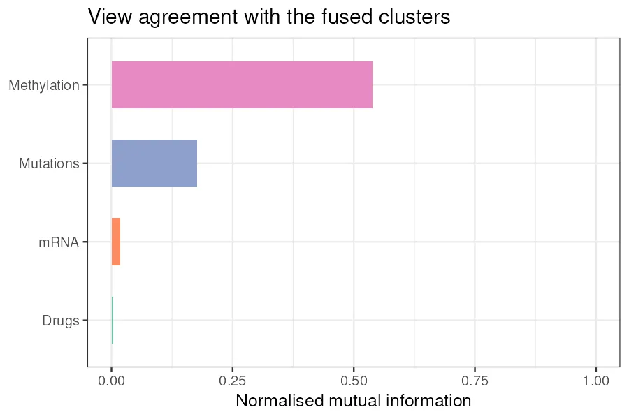
Methylation carries the fusion, at NMI 0.54, with mutations a distant second at 0.18 and expression and drug response contributing almost nothing to the patient grouping. That matches CLL biology: the IGHV split has a strong epigenetic signature, and SNF finds it through the methylation layer.

A caveat worth stating

The clusters recover IGHV almost perfectly, yet the mean silhouette of the fused clustering is 0.004, essentially zero. Internal cluster-compactness indices and biological validity disagree here. The fused similarity is smooth rather than sharply blocky, so a silhouette score sees weak separation while the biology sees a clean split. Trust the biological readout, IGHV, over the geometry of the fused distance, and do not reject an SNF result because a silhouette looks poor.

Where SNF stops

SNF returns clusters and nothing else. It does not tell you which genes, CpGs, or mutations separate the groups; for that you run a differential analysis on top of the labels. It also asks you to choose the number of clusters, so pick K deliberately and check the result against known biology rather than reading it off a silhouette. When you need the driving features rather than the grouping, reach for MOFA or DIABLO.

The runnable script and the container are in the companion code repo under guides/multi-omics/snf/.