Multiple Testing Correction

A p-value of 0.05 means a 5% chance of a false positive per test. Run one test and that is fine. Run 20,000, one per gene, and you expect a thousand false positives by chance alone. Multiple testing correction is what makes genome-scale statistics honest. This page corrects 1000 gene tests, in R and Python.

Every code block on this page runs in a container in the companion repository. The numbers and figures come from those real runs.

When to correct

Correct whenever you test many hypotheses and report the significant ones: differential expression across genes, association across variants, enrichment across pathways. Any time you scan and pick winners, the raw p-values are not trustworthy on their own.

The data

pvalues.csv holds one p-value per gene for 1000 genes. By construction 900 are true nulls and 100 have a real effect, though in real data you never know which.

Read the p-value histogram first

Before correcting, plot the p-values. A healthy result is a flat uniform background, from the nulls, with a spike near zero, from the true effects. Anything else, such as a hump in the middle, signals a modelling problem upstream.

R

library(ggplot2)

ggplot(df, aes(pvalue)) +
  geom_histogram(binwidth = 0.05, boundary = 0)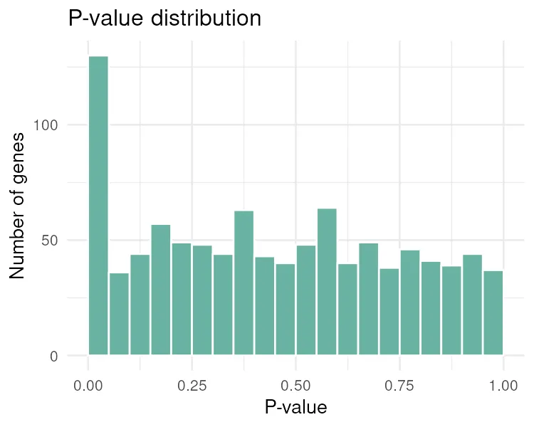

Python

import seaborn as sns

sns.histplot(df["pvalue"], binwidth=0.05)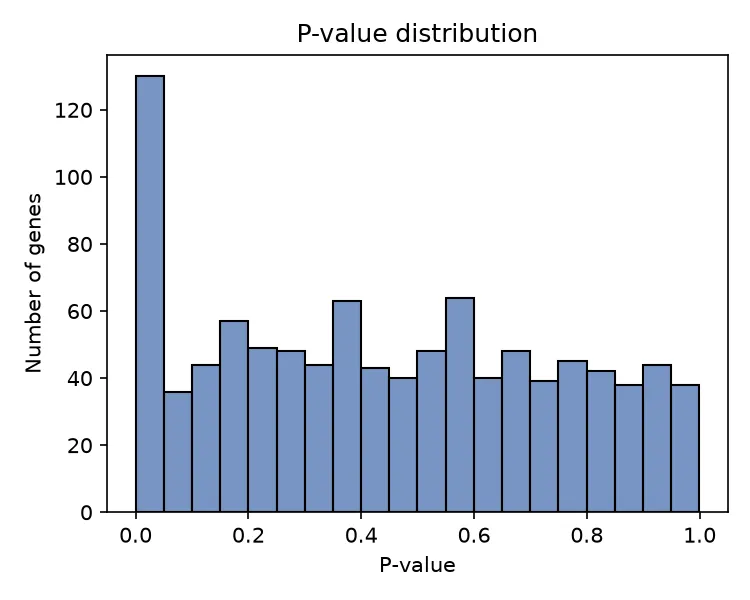

The spike in the first bin is the real signal. The flat rest is the null. That spike is what correction tries to recover without dragging along the noise.

Raw, Bonferroni, and FDR

Three rules, from reckless to strict to balanced.

R

p <- df$pvalue
sum(p < 0.05)                          # raw
sum(p.adjust(p, "bonferroni") < 0.05)  # Bonferroni, controls FWER
sum(p.adjust(p, "BH") < 0.05)          # Benjamini-Hochberg, controls FDR

Raw p < 0.05:        130
Bonferroni < 0.05:   18
BH / FDR < 0.05:     43

Python

from statsmodels.stats.multitest import multipletests

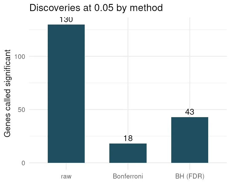
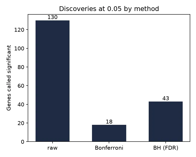
p = df["pvalue"].values
(p < 0.05).sum()
multipletests(p, method="bonferroni")[0].sum()
multipletests(p, method="fdr_bh")[0].sum()

Raw p < 0.05:        130
Bonferroni < 0.05:   18
BH / FDR < 0.05:     43

Both languages give the same counts. The raw rule calls 130 genes, but around 45 of those are false positives from the 900 nulls. The corrections rein that in.

• Bonferroni controls the family-wise error rate, the chance of even one false positive. It multiplies each p-value by the number of tests. Safe but harsh: only 18 genes survive, and many true effects are lost.
• Benjamini-Hochberg controls the false discovery rate, the expected fraction of false positives among the genes you call. It calls 43 genes, accepting a small, known share of false positives to keep many more true ones.

R

Python

Pitfalls and bioinformatics notes

• FDR, not FWER, for discovery. In genomics you want a list worth following up, not a guarantee of zero errors. Benjamini-Hochberg is the field standard; DESeq2 and edgeR report BH-adjusted p-values by default.
• Report the adjusted value, and say which. “FDR < 0.05” and “Bonferroni < 0.05” mean very different things. Name the method.
• Correct over the whole family. Adjust across all genes you tested, not just the ones that looked interesting. Cherry-picking the family breaks the guarantee.
• A weird histogram means fix the model, not the threshold. A hump near one or a slope means the p-values are miscalibrated. Correction cannot rescue that.

Key points

• Testing many hypotheses at 0.05 produces false positives in proportion to the number of tests.
• Bonferroni controls the chance of any false positive; it is strict.
• Benjamini-Hochberg controls the false discovery rate; it is the genomics default.
• Always plot the p-value histogram, and always report which correction you used.

Further reading

• Benjamini and Hochberg (1995), the original FDR paper.
• The previous guides, Two groups and ANOVA, for the tests that produce these p-values.