Feature Selection

Feature selection removes uninformative or redundant features. This reduces overfitting, speeds up training, and can improve performance. Here we compare five approaches on a synthetic dataset with 20 features, 8 of them informative.

Every code block runs in a container in the companion repository, so the numbers are real.

Setup

import numpy as np
import pandas as pd
from sklearn.datasets import make_classification

X, y = make_classification(n_samples=500, n_features=20, n_informative=8,
                           n_redundant=2, random_state=42)
feature_names = [f"feature_{i}" for i in range(X.shape[1])]

Variance thresholding

The simplest filter. Features with near-zero variance carry no information.

from sklearn.feature_selection import VarianceThreshold

rng = np.random.RandomState(42)
X_noisy = np.column_stack([X, rng.normal(0, 0.001, (500, 5))])

selector = VarianceThreshold(threshold=0.01)
X_filtered = selector.fit_transform(X_noisy)
print(f"Features before: {X_noisy.shape[1]}, after: {X_filtered.shape[1]}")

Features before: 25, after: 20

All five near-zero-variance noise columns are removed.

Univariate selection

Univariate methods score each feature independently against the target.

The F-test (ANOVA) measures whether a feature’s mean differs between classes:

from sklearn.feature_selection import SelectKBest, f_classif

sel = SelectKBest(f_classif, k=10).fit(X, y)
pd.DataFrame({"feature": feature_names, "f_score": sel.scores_,
             "p_value": sel.pvalues_}).sort_values("f_score", ascending=False).head(6)

   feature   f_score      p_value
feature_16 60.224901 4.834258e-14
feature_18 50.742350 3.709522e-12
feature_13 29.243132 9.926065e-08
 feature_5 22.595704 2.620671e-06
 feature_6  4.321873 3.813677e-02
 feature_7  4.307767 3.845142e-02

Mutual information captures nonlinear associations the F-test misses:

from sklearn.feature_selection import mutual_info_classif

mi = mutual_info_classif(X, y, random_state=42)
pd.DataFrame({"feature": feature_names, "mi_score": mi}).sort_values(
    "mi_score", ascending=False).head(5)

   feature  mi_score
feature_16  0.055935
feature_13  0.051800
 feature_5  0.049058
feature_18  0.033025
 feature_6  0.021969

Recursive feature elimination

RFE trains a model, drops the least important feature, and repeats. Unlike univariate methods, it accounts for feature interactions.

from sklearn.feature_selection import RFE
from sklearn.linear_model import LogisticRegression
from sklearn.preprocessing import StandardScaler

rfe = RFE(LogisticRegression(max_iter=1000, random_state=42),
          n_features_to_select=10).fit(StandardScaler().fit_transform(X), y)

RFE selects feature_1 and feature_3, which the univariate methods ranked low: they become informative only in combination with others.

Tree-based importance

Random forests compute importance as a byproduct of training.

from sklearn.ensemble import RandomForestClassifier

rf = RandomForestClassifier(n_estimators=100, random_state=42).fit(X, y)
pd.DataFrame({"feature": feature_names,
             "importance": rf.feature_importances_}).sort_values(
    "importance", ascending=False).head(6)

   feature  importance
feature_16    0.134316
feature_18    0.118628
 feature_5    0.097055
feature_13    0.087026
feature_15    0.068941
 feature_4    0.048066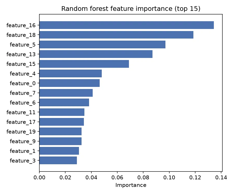

The top four features (16, 18, 5, 13) rank high by every method, a strong signal they carry real information.

Importance bias

Random forest importance is biased toward high-cardinality features. For a fairer measure, use permutation importance, which shuffles each feature and measures the drop in performance.

LASSO-based selection

L1 regularization shrinks some coefficients to exactly zero, removing those features. In current scikit-learn, request pure L1 with l1_ratio=1.

lasso = LogisticRegression(solver="saga", l1_ratio=1, C=0.1,
                           max_iter=5000, random_state=42)
lasso.fit(StandardScaler().fit_transform(X), y)
print(f"Non-zero features: {(lasso.coef_[0] != 0).sum()} / {len(feature_names)}")

Non-zero features: 11 / 20

LASSO kept 11 features and zeroed 9. The coefficient sign gives the direction: feature_16 is positive (raises the probability of class 1), feature_18 negative.

Does selection help?

Compare cross-validated ROC-AUC with all 20 features versus the top 10 by importance.

from sklearn.model_selection import cross_val_score, StratifiedKFold, train_test_split
from sklearn.pipeline import Pipeline

X_train, X_test, y_train, y_test = train_test_split(
    X, y, test_size=0.2, stratify=y, random_state=42)
cv = StratifiedKFold(n_splits=5, shuffle=True, random_state=42)
pipe = Pipeline([("scaler", StandardScaler()),
                 ("clf", LogisticRegression(max_iter=1000, random_state=42))])

top10_idx = [feature_names.index(f) for f in
             pd.Series(rf.feature_importances_, feature_names).nlargest(10).index]
print("All 20:", cross_val_score(pipe, X_train, y_train, cv=cv, scoring="roc_auc").mean())
print("Top 10:", cross_val_score(pipe, X_train[:, top10_idx], y_train, cv=cv, scoring="roc_auc").mean())

All 20 features: ROC-AUC = 0.8088 (+/- 0.0336)
Top 10 features: ROC-AUC = 0.8246 (+/- 0.0261)

Dropping the ten least important features lifted ROC-AUC from 0.81 to 0.82 and reduced variance. The noise was hurting the model.

Which method to use

Method	Speed	Interactions	Good for
Variance threshold	Very fast	No	First pass, remove constants
F-test / mutual info	Fast	No / Yes	Quick ranking of many features
RFE	Slow	Yes	Careful selection, smaller data
Tree importance	Fast	Yes	Quick ranking with any tree model
LASSO	Fast	No	Selection and modeling at once

Select inside cross-validation

Always run feature selection inside cross-validation. Selecting on the full dataset and then cross-validating leaks the validation data into the selection step.

Next steps

The next page covers Feature Engineering: creating new features to give the model more signal.