Detecting Batch Effects

You cannot decide how to handle a batch you have not seen. The cheapest honest look at one is a PCA of the variance-stabilized counts, colored by condition and shaped by batch, because a batch effect that moves counts shows up as samples grouping by batch, and a batch effect that leaves no trace needs no correction. This page builds that plot for the pasilla data and reads what it says.

The transformed matrix

The pipeline is the one the RNA-seq QC page teaches: filter genes with almost no reads, then apply the variance-stabilizing transformation, so that distances between samples reflect the samples rather than the size of their libraries.

library(DESeq2)
library(pasilla)

# Counts and annotation, loaded the way the DESeq2 vignette does.
pas_anno <- system.file("extdata", "pasilla_sample_annotation.csv",
                        package = "pasilla", mustWork = TRUE)
coldata <- read.csv(pas_anno, row.names = 1)
coldata <- coldata[, c("condition", "type")]
rownames(coldata) <- sub("fb", "", rownames(coldata))
coldata$condition <- relevel(factor(coldata$condition), ref = "untreated")

pas_cts <- system.file("extdata", "pasilla_gene_counts.tsv",
                       package = "pasilla", mustWork = TRUE)
cts <- as.matrix(read.csv(pas_cts, sep = "\t", row.names = "gene_id"))
cts <- cts[, rownames(coldata)]

# Keep genes with at least 10 reads total.
keep <- rowSums(cts) >= 10
cts <- cts[keep, ]

dds <- DESeqDataSetFromMatrix(cts, coldata, design = ~ condition)
vsd <- vst(dds, blind = TRUE)

PCA

plotPCA projects the samples onto the first two principal components of the 500 most variable genes. With returnData = TRUE it hands back the coordinates instead of drawing, so the numbers can be read before the plot is drawn.

# PCA coordinates, with condition and type attached per sample.
pca_data <- plotPCA(vsd, intgroup = c("condition", "type"),
                    returnData = TRUE)
pca_data[, c("PC1", "PC2", "condition", "type")]

# The fraction of the total variance on each axis.
attr(pca_data, "percentVar")

                  PC1       PC2 condition        type
treated1    -8.391959 10.763545   treated single-read
treated2   -11.314585 -2.676609   treated  paired-end
treated3   -11.347261 -4.768213   treated  paired-end
untreated1   9.118926  6.698109 untreated single-read
untreated2   8.921845  4.173830 untreated single-read
untreated3   6.586707 -7.405149 untreated  paired-end
untreated4   6.426326 -6.785513 untreated  paired-end
[1] 0.5648530 0.3036567

The first axis carries 56 percent of the variance and separates treated from untreated samples, which is the biology. The second axis carries 30 percent and separates single-read from paired-end libraries, which is the batch. Of the two largest sources of variation in this matrix, one is the knockdown and one is the library protocol.

That 30 percent is worth a pause. The batch is not a small nuisance sitting behind the biology. It is the second largest source of variation in the counts, ahead of anything else the data contains, and a differential expression model that ignores it folds all of it into the residual variance.

The figure

library(ggplot2)

percent_var <- round(100 * attr(pca_data, "percentVar"))

pca_plot <- ggplot(pca_data, aes(PC1, PC2, color = condition, shape = type)) +
  geom_point(size = 4) +
  xlab(paste0("PC1: ", percent_var[1], "% variance")) +
  ylab(paste0("PC2: ", percent_var[2], "% variance")) +
  scale_color_manual(values = c(untreated = "#2166ac", treated = "#b2182b")) +
  theme_minimal()

ggsave("outputs/batch-pca.png", pca_plot, width = 6, height = 4.5,
       dpi = 150, bg = "white")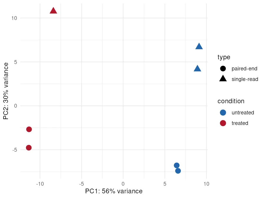

Color carries the condition and shape carries the batch, so a sample in the wrong group would be visible twice over. The plot shows the clean version of a confounded study. If instead the shapes had clustered on the first axis and the colors had mixed, the batch would be the dominant signal and the condition comparison would be in trouble before any model ran.

The next two pages take the two standard routes from here. The design route leaves the matrix untouched and adds one term to the model. The removal route rewrites the matrix with ComBat and is the right tool in a narrower set of situations than its popularity suggests.