ANCOVA, Adjusting for a Covariate

The question

Three arms of a mouse study, control, low dose and high dose, and tumour volume measured at the end. Do the arms differ?

A one-way ANOVA answers that in one line and, on this data, gets it wrong. Randomisation was imperfect: the dosed arms started with larger tumours. Baseline volume carries forward, so it masks the treatment effect. ANCOVA is the ANOVA that accounts for it.

Every code block on this page runs in a container in the companion repository. The numbers and figures come from those real runs.

When to use it, and when not to

Use ANCOVA when you are comparing groups and you have a continuous variable that also affects the outcome. Two distinct reasons to reach for it:

Correction. The covariate is imbalanced across groups, so the raw comparison is confounded. That is this page.
Precision. The covariate is balanced but predictive, so adjusting for it removes noise and shrinks the standard errors. In a randomised trial with a baseline measurement, this is the usual reason, and it is worth doing even when the arms look balanced.

Do not use ANCOVA when the covariate is affected by the treatment. Adjusting for something downstream of the intervention adjusts away part of the effect you are trying to measure. Baseline values recorded before randomisation are safe; anything measured after is not.

And do not use it when the groups have genuinely different slopes. That is a real finding, not a nuisance, and it needs an interaction model instead.

ANCOVA is not a separate technique from multiple regression. It is a linear model with one categorical predictor and one continuous one. The name is a convention from the experimental-design literature, and the machinery is identical.

The data

tumour_trial.csv, 30 mice per arm, 90 rows, with baseline_volume and final_volume.

The imbalance is severe and deliberate. Mean baseline volume runs 99.6 in control, 114.1 in low dose and 128.2 in high dose, and a test of baseline across arms returns p = 9.7e-14. Baseline carries through to the final volume at about 0.85 per unit, which very nearly cancels the true treatment effects of -12 and -26.

The result is a trap: the arms finish at 125.9, 126.1 and 122.2. Nearly identical.

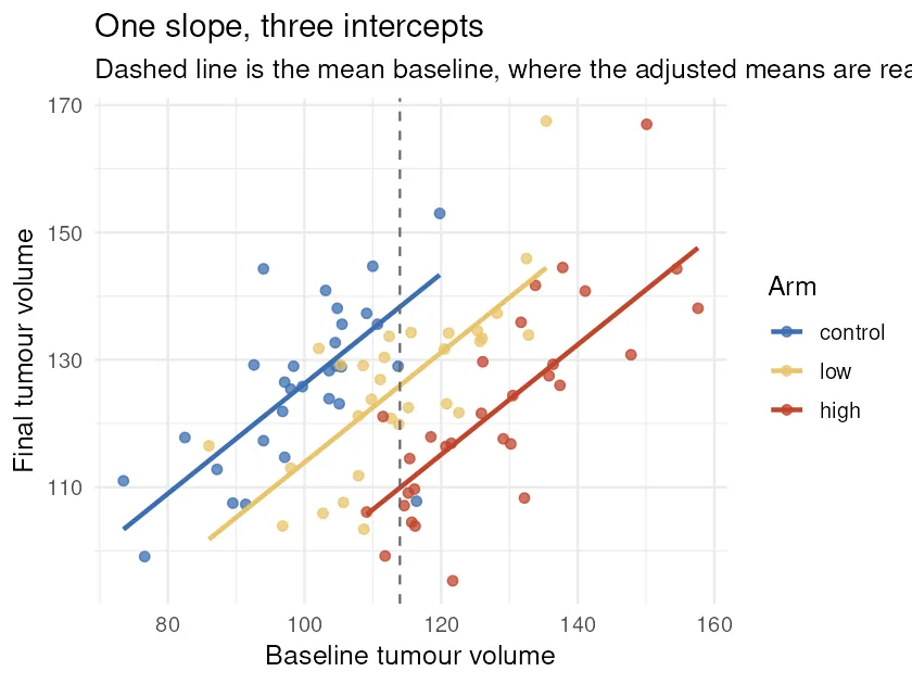
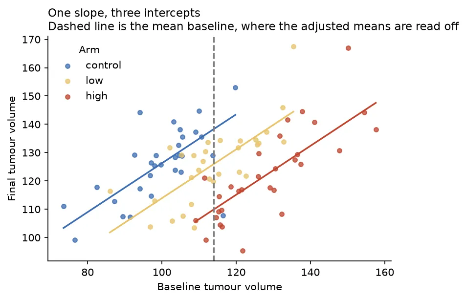
Assumptions and how to check them

ANCOVA fits one common slope for the covariate and lets only the intercepts differ between groups. That is the assumption worth checking, and it has a name: homogeneity of slopes.

Test it by comparing the additive model with the interaction model. If the interaction matters, the arms respond differently to baseline and a single adjusted effect is not a meaningful summary.

Here the interaction gives p = 0.560. The slopes are common and ANCOVA is appropriate. The other assumptions are the ordinary linear-model ones: normal residuals, constant variance, independence.

library(car)       # Anova() with Type II sums of squares
library(emmeans)   # covariate-adjusted marginal means

df <- read.csv("tumour_trial.csv")
df$arm <- factor(df$arm, levels = c("control", "low", "high"))

# 1. The unadjusted answer, which is wrong.
summary(aov(final_volume ~ arm, data = df))

# 2. Homogeneity of slopes: additive versus interaction.
add_fit <- lm(final_volume ~ arm + baseline_volume, data = df)
int_fit <- lm(final_volume ~ arm * baseline_volume, data = df)
anova(add_fit, int_fit)

# 3. The ANCOVA. Type II so the arm effect is tested AFTER baseline.
Anova(add_fit, type = 2)

# 4. Adjusted means, evaluated at the study-wide mean baseline.
emm <- emmeans(add_fit, ~ arm)
emm
pairs(emm)

import pandas as pd
import statsmodels.formula.api as smf
from statsmodels.stats.anova import anova_lm

ARMS = ["control", "low", "high"]
df = pd.read_csv("tumour_trial.csv")
df["arm"] = pd.Categorical(df["arm"], categories=ARMS)

# 1. The unadjusted answer, which is wrong.
anova_lm(smf.ols("final_volume ~ C(arm)", data=df).fit(), typ=2)

# 2. Homogeneity of slopes: additive versus interaction.
add_fit = smf.ols("final_volume ~ C(arm) + baseline_volume", data=df).fit()
int_fit = smf.ols("final_volume ~ C(arm) * baseline_volume", data=df).fit()
anova_lm(add_fit, int_fit)

# 3. The ANCOVA.
anova_lm(add_fit, typ=2)

# 4. Adjusted means. There is no emmeans in Python, so do what emmeans does:
#    predict every arm at the study-wide mean of the covariate.
grid = pd.DataFrame({
    "arm": pd.Categorical(ARMS, categories=ARMS),
    "baseline_volume": df["baseline_volume"].mean(),
})
add_fit.get_prediction(grid).summary_frame(alpha=0.05)

Reading the output

The unadjusted ANOVA gives F = 0.73, p = 0.487. No evidence of any difference. On this data that conclusion is wrong, and nothing in the output hints at it.

The ANCOVA gives F = 32.97, p = 2.3e-11 for the arm effect, with a baseline slope of 0.863, close to the 0.85 the data was built with.

The adjusted means are where the result actually lives. All three are evaluated at the study-wide mean baseline of 113.97, which is the “what if the arms had started equal” question:

arm	raw mean	adjusted mean	95% CI
control	125.92	138.31	134 to 143
low	126.06	125.95	122 to 129
high	122.20	109.91	106 to 114

The raw means span 3.9 units and say nothing. The adjusted means span 28.4 and show a clean dose-response. Tukey-adjusted contrasts: control minus low is 12.4 (p = 0.0001), control minus high is 28.4 (p < 0.0001), low minus high is 16.0 (p < 0.0001).

Two details worth knowing. Type II sums of squares test the arm effect after accounting for baseline, so the order of terms in the formula stops mattering; with a Type I table, arm + baseline and baseline + arm give different answers. And adjusted means are a model prediction, not a summary of the data. Report the covariate value they were evaluated at, because they change if you move it.

Visualizing it

Two figures do the work. The first shows what ANCOVA assumes and estimates: one slope, three intercepts, with the dashed line marking the baseline where the adjusted means are read off.

R
Python

Scatter of final against baseline volume with three parallel fitted lines, one per arm (R)

Raw group means side by side with baseline-adjusted means, the raw ones overlapping and the adjusted ones separated (R)

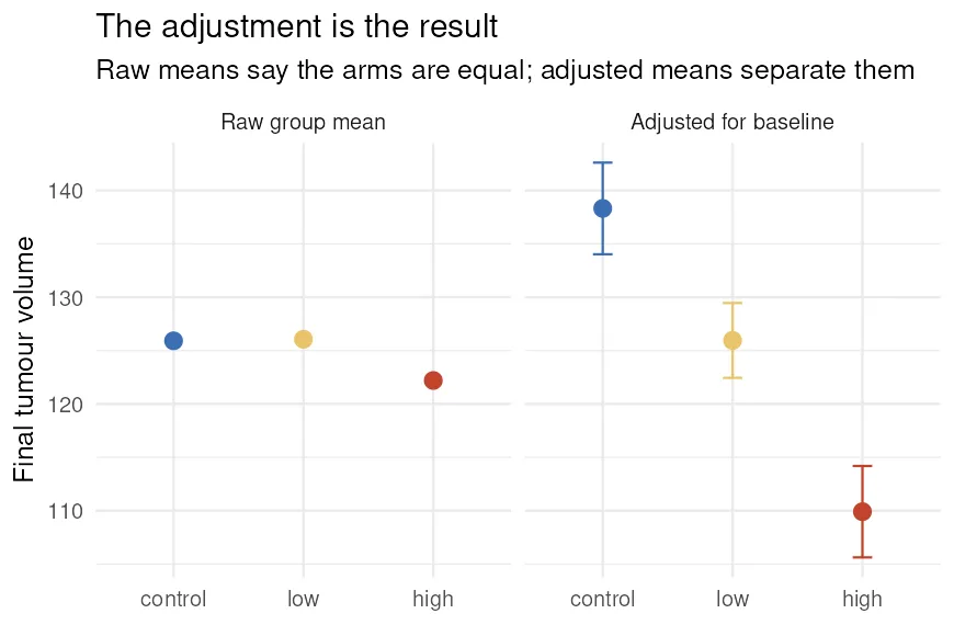
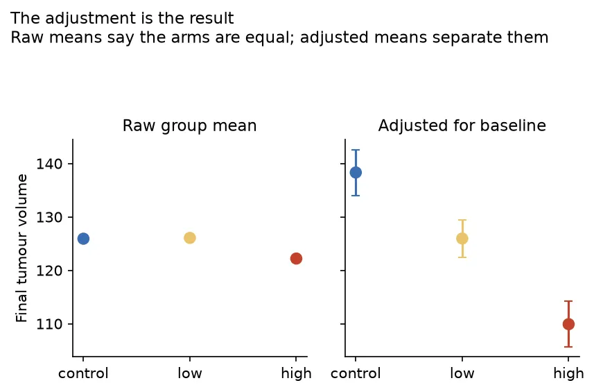
The second figure is the argument of the page in one image. On the left the three arms sit on top of each other. On the right they separate cleanly, and nothing changed but the adjustment.

Pitfalls and bioinformatics notes

Never adjust for a post-treatment variable. If the covariate is downstream of the intervention, adjusting removes part of the effect. Baseline measured before randomisation is safe.
Check the slopes before you trust one adjusted effect. If the interaction is significant, the honest report is the interaction, not a single adjusted difference.
Adjusted means require overlap. They are evaluated at one covariate value, and if the arms barely overlap on the covariate the model is extrapolating for at least one of them. Plot the covariate by group before believing the adjustment.
Change scores are not the same thing. Analysing final - baseline looks similar but assumes the slope is exactly 1. Here it is 0.863, and ANCOVA is more powerful whenever the true slope is not 1. This is Lord’s paradox territory: the two analyses can disagree, and ANCOVA on the final value is the standard choice for randomised trials.
The same pattern shows up as batch in omics. Comparing conditions when batch is confounded with condition is this page’s problem with a categorical covariate, and it is why experimental design beats statistical rescue.

Key points

ANCOVA compares group means adjusted for a continuous covariate.
Here the unadjusted ANOVA gave p = 0.487 and the adjusted one gave p = 2.3e-11 on the same data.
Check homogeneity of slopes by testing the interaction. Here p = 0.560, so a single slope is fair.
Use Type II sums of squares so the arm effect is tested after the covariate.
Report adjusted means with the covariate value they were evaluated at.
R has emmeans. Python does not, so predict at the covariate mean by hand; the two agree to floating point.