Generalized Mixed Models

The question

A pathologist scores six biopsy sites per patient for a marker, present or absent, in 40 patients. Does dose raise the odds of a site being positive?

The outcome is binary, so it needs a logit link. The sites are clustered inside patients, so they are not 240 independent observations. Put those together and you need a generalized linear mixed model: the “generalized” handles the binary outcome, the “mixed” handles the clustering.

Every code block on this page runs in a container in the companion repository. The numbers and figure come from those real runs.

When to use it, and when not to

Use a GLMM when both things are true: the outcome is not continuous, and the observations are grouped. Binary calls per patient, cell counts per animal, positive wells per plate, reads per sample within a batch.

If the outcome is continuous and grouped, you want a plain linear mixed model, which the Mixed-Effects guide covers. If the outcome is binary and the observations really are independent, ordinary logistic regression is correct and simpler.

The wrong choice this replaces is pooling. Throwing all 240 rows into a logistic regression treats six correlated sites as six independent pieces of evidence, which manufactures confidence that the study never earned.

The data

biopsy_marker.csv, 40 patients by 6 sites, 240 rows, 55.4% positive overall. Dose is assigned per patient, at 0, 1 or 2, so the real sample size for the dose question is much closer to 40 than to 240.

The fixture is built with a between-patient SD of 1.5 on the log-odds scale. That is large on purpose: patients differ from each other far more than dose moves any single patient. Per-patient positive rates run from 0.00 to 1.00.

Assumptions and how to check them

The random intercept assumes patient effects are normal on the log-odds scale, and that the clustering is captured by a single per-patient shift.

The first thing to check is whether clustering matters at all, and the model itself answers it. The fitted between-patient SD is 1.106, giving an intraclass correlation of 0.271: 27% of the latent variance is between patients rather than within them. That is not ignorable.

Cluster size matters for the fit. With only 6 sites per patient the default Laplace approximation is noticeably biased, so the R fit below uses nAGQ = 10, adaptive Gauss-Hermite quadrature with ten points.

library(lme4)

df <- read.csv("biopsy_marker.csv")
df$patient <- factor(df$patient)

# The naive model, for contrast: 240 rows treated as independent.
naive <- glm(marker_positive ~ dose, family = binomial, data = df)

# The GLMM. (1 | patient) gives each patient its own baseline log-odds.
# nAGQ = 10 uses adaptive Gauss-Hermite quadrature rather than the default
# Laplace approximation, which is biased when clusters are small.
fit <- glmer(marker_positive ~ dose + (1 | patient), family = binomial,
             data = df, nAGQ = 10)
summary(fit)

patient_sd <- sqrt(as.numeric(VarCorr(fit)$patient))
# The logistic residual variance is pi squared divided by three.
icc <- patient_sd^2 / (patient_sd^2 + pi^2 / 3)

import pandas as pd
import statsmodels.api as sm
import statsmodels.formula.api as smf

df = pd.read_csv("biopsy_marker.csv")

# The naive model, for contrast: 240 rows treated as independent.
naive = smf.glm("marker_positive ~ dose",
                data=df,
                family=sm.families.Binomial()).fit()

# statsmodels has no frequentist binomial GLMM. GEE is the mainstream Python
# answer for clustered binary data. groups= names the cluster; the exchangeable
# structure says any two sites from one patient are equally correlated, which is
# the GEE analogue of a random intercept.
# Standard errors use sandwich estimates.
gee = smf.gee(
    "marker_positive ~ dose",
    groups="patient",
    data=df,
    family=sm.families.Binomial(),
    cov_struct=sm.cov_struct.Exchangeable(),
).fit()
gee.summary()

Reading the output

Three models, three answers.

model	log-odds per dose	SE	what it estimates
Naive pooled logistic	0.7195	0.1559	nothing trustworthy
glmer, R	0.9009	0.2746	subject-specific (conditional)
GEE, Python	0.7195	0.2204	population-averaged (marginal)

Look at the standard errors first. Respecting the clustering costs a factor of 1.76 in R and 1.41 in Python. The naive model’s confidence was borrowed against observations it did not have.

Now the part that surprises people. glmer and GEE return different coefficients, and that is correct. They estimate different quantities:

glmer gives the conditional effect: how one patient’s log-odds change if their dose goes up a level.
GEE gives the marginal effect: how the log-odds shift across the whole population if everyone moved up a level.

For a logit link those are not the same number, and the marginal one is always attenuated toward zero. The standard approximation divides the conditional effect by sqrt(1 + 0.346 * sigma^2). With sigma = 1.106 that factor is 1.193, so glmer’s 0.9009 predicts a marginal effect of 0.7552. GEE returned 0.7195. The two languages land within 5% of each other, on a difference that theory says should be there.

So this page does not compare glmer and GEE in its build gate. It compares the naive pooled model, which both languages fit identically, and it says plainly why the other two differ.

Which one to report depends on the question. A clinician asking “what happens if I raise this patient’s dose” wants the conditional effect. A policy question about a whole population wants the marginal one.

Visualizing it

Per-patient positive rates within each dose level. If dose explained the variation, each dose would show a tight band. It does not: patients span the full range inside every dose level.

R
Python

Per-patient positive rates by dose level, spread across the full range within every level (R)

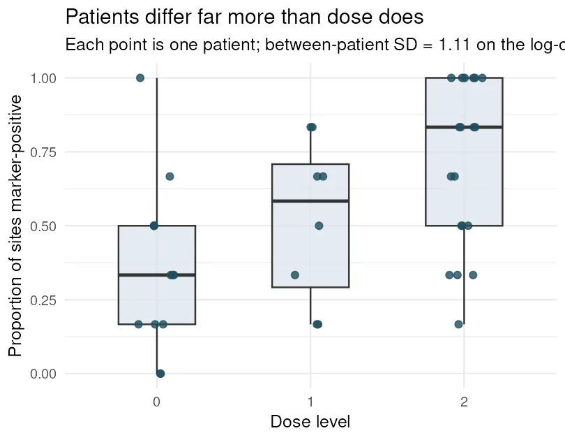
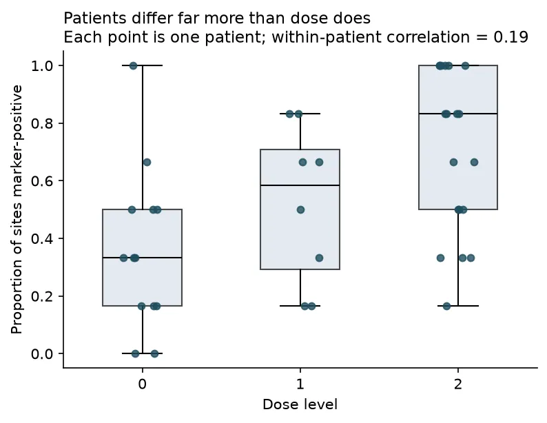
Each point is a patient, not a site. Plotting one point per patient rather than 240 per figure is itself the honest move: it shows the sample size the dose question actually has.

Pitfalls and bioinformatics notes

Do not compare a glmer coefficient with a GEE coefficient and call the difference a bug. Check the attenuation factor first. Comparing a conditional estimate from one paper with a marginal one from another is a real and common error.
Laplace is the default and it is biased for small clusters. With a handful of observations per group, set nAGQ to 10 or so. It costs nothing here and it changes the estimate.
Convergence warnings mean something. glmer frequently warns on random-effect structures the data cannot support. Simplify the random effects rather than suppressing the warning.
Python’s gap is real, not a search failure. statsmodels ships GEE and a variational Bayes mixed GLM, but no frequentist binomial GLMM comparable to glmer. If you need the conditional estimate in a Python pipeline, call R.
At genome scale the same structure appears as a random effect per subject in single-cell differential expression. Treating cells from one donor as independent replicates is the same error as treating six sites from one patient as independent, and it inflates significance the same way.

Key points

Non-Gaussian outcome plus clustering means a GLMM.
Pooling gave a standard error 1.76 times too small here.
The ICC of 0.271 says over a quarter of the latent variance is between patients.
glmer estimates a conditional effect, GEE a marginal one. The gap is predictable from the random-effect SD, and here prediction and observation agreed to within 5%.
Say which one you are reporting.