Clustering
Gating names the populations before it finds them. You decide there are T cells, then draw a gate for them. Clustering does the reverse: it groups events by the shape of their marker profile and lets the populations emerge from the data. FlowSOM is the standard tool, a self-organizing map that compresses the events into a grid of nodes and then meta-clusters the nodes into populations.
Why clustering and not gating
Section titled “Why clustering and not gating”Gating is interpretable and slow. You draw one gate at a time, and a 40-marker panel has hundreds of biaxial plots. Clustering is fast and unsupervised, and it finds populations a gate sequence would miss, because it does not commit to an order. The cost is that the clusters are not named until you annotate them, by looking at the median marker intensity in each cluster and calling it a cell type.
FlowSOM on the Bodenmiller panel
Section titled “FlowSOM on the Bodenmiller panel”The Bodenmiller BCR-XL data ships in HDCytoData on the raw scale. The example
arcsinh-transforms the surface markers, the channels whose names start with CD, and
asks FlowSOM for eight metaclusters.
library(flowCore)library(FlowSOM)library(HDCytoData)
fs <- Bodenmiller_BCR_XL_flowSet()markers <- grep("^CD", colnames(fs[[1]]), value = TRUE)
# Keep the untransformed events before transforming, because the Python tab# below applies its own transform and must not be handed transformed values.raw <- do.call(rbind, lapply(seq_len(length(fs)), function(i) {  exprs(fs[[i]])[, markers, drop = FALSE]}))
# Arcsinh-transform the surface CD markers (cofactor 5).asinh_trans <- arcsinhTransform(a = 0, b = 1 / 5, c = 0)fs <- transform(fs, transformList(markers, tfun = asinh_trans))markers
set.seed(1)fom <- FlowSOM(fs, colsToUse = markers, nClus = 8, seed = 1)
# The number of metaclusters FlowSOM settled on.length(unique(fom$metaclustering))
# Hand the untransformed events to the Python tab, so both engines cluster the# same cells and each applies its own transform. 20000 of the 172791 events,# sampled with a seed, keeps the page quick.dir.create("outputs", showWarnings = FALSE, recursive = TRUE)set.seed(1)keep <- sort(sample(nrow(raw), 20000))write.csv(raw[keep, ], "outputs/cluster_events.csv", row.names = FALSE)nrow(raw)
[1] "CD3(110:114)Dd" "CD45(In115)Dd" "CD4(Nd145)Dd" "CD20(Sm147)Dd"[5] "CD33(Nd148)Dd" "CD123(Eu151)Dd" "CD14(Gd160)Dd" "CD7(Yb176)Dd"[1] 8[1] 172791FlowSOM() builds the self-organizing map, assigns every event to a node, and
meta-clusters the nodes into the requested number of populations. The
metaclustering vector holds one label per SOM node. The number of distinct labels is
the number of populations the algorithm found.
Cluster medians
Section titled “Cluster medians”A cluster is identified by its median marker intensity. The table below is the annotation step: you read the medians and call each cluster a cell type.
# The SOM codebook: one row per node, one column per marker. FlowSOM 2.x# returns a flat object, so the map sits at the top level.node_codes <- fom$map$codesdim(node_codes)
# Median intensity per metacluster, across the surface markers.meta <- fom$metaclusteringcluster_medians <- t(sapply(sort(unique(meta)), function(g) {  apply(node_codes[meta == g, , drop = FALSE], 2, median)}))round(cluster_medians, 2)
[1] 100 8 CD3(110:114)Dd CD45(In115)Dd CD4(Nd145)Dd CD20(Sm147)Dd CD33(Nd148)Dd[1,] 3.50 5.41 3.63 0.17 0.09[2,] 1.40 5.29 2.24 0.85 0.50[3,] 1.28 5.14 0.08 0.11 0.03[4,] 1.87 5.36 0.60 0.23 1.40[5,] 2.11 5.32 0.18 0.13 0.04[6,] -0.10 2.21 0.16 0.16 0.07[7,] 0.99 3.62 0.62 0.39 0.34[8,] 0.23 5.02 0.25 4.23 0.59 CD123(Eu151)Dd CD14(Gd160)Dd CD7(Yb176)Dd[1,] -0.08 0.06 2.79[2,] 0.23 0.43 0.11[3,] -0.08 0.18 3.79[4,] 2.25 1.39 0.49[5,] -0.08 0.11 0.25[6,] 0.13 0.40 0.23[7,] 4.25 0.76 0.57[8,] 0.06 0.36 0.28Cluster 1 is high on CD3, CD4 and CD7, which is a CD4 T cell. Cluster 8 is the only one high on CD20, so it is the B cell cluster, and the BCR-XL stimulation in this dataset acts on those cells. Cluster 4 carries CD33, CD123 and CD14 together, which is myeloid. Cluster 6 sits low on everything including CD45, so it is debris rather than a cell type. The medians are the evidence; the names are the interpretation you write beside them.
A UMAP projection
Section titled “A UMAP projection”FlowSOM’s nodes live in a high-dimensional marker space. A UMAP projection drops them into two dimensions so you can see how the clusters relate, which ones sit close because they share markers and which ones sit apart.
library(uwot)
set.seed(1)node_umap <- umap(node_codes, n_neighbors = 8, min_dist = 0.1, seed = 1)head(node_umap)
[,1] [,2][1,] -4.597413 -0.51866809[2,] -5.577594 0.09192019[3,] -4.634599 -0.66788874[4,] -5.161691 -0.42374516[5,] -4.714157 0.03685798[6,] -3.756753 -0.53402088library(ggplot2)
dir.create("outputs", showWarnings = FALSE, recursive = TRUE)
umap_df <- data.frame( umap1 = node_umap[, 1], umap2 = node_umap[, 2], metacluster = factor(meta))
umap_plot <- ggplot(umap_df, aes(x = umap1, y = umap2, color = metacluster)) + geom_point(size = 2.5, alpha = 0.9) + labs( title = "The 100 SOM nodes, coloured by metacluster", x = "UMAP 1", y = "UMAP 2" ) + theme_minimal()
ggsave("outputs/cyto-umap-nodes.png", plot = umap_plot, width = 6, height = 5, dpi = 110, bg = "white")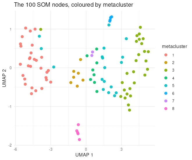
Four of the eight metaclusters sit in their own region, which is what you hope to see. Metaclusters 4 and 5 do not. They interleave through the middle of the projection, and a few of the metacluster 5 nodes sit inside metacluster 1 on the far left.
That is the honest part of the picture. The boundary between two populations is a gradient, the metaclustering step had to cut it somewhere, and the cut it made does not correspond to a gap in the data. A table of medians would have shown eight tidy rows and hidden this completely.
The projection is of the SOM nodes, not the raw events, so it is fast even on a large file. Each point is a node, coloured by its metacluster. The clustering page and the gating page are two answers to the same question, and a real study uses both: gating for the populations you already know, clustering for the ones you do not.
The same clustering in Python
Section titled “The same clustering in Python”R is where the cytometry stack lives, but it is not the only place FlowSOM exists.
pytometry puts a cytometry layer on top of AnnData and scanpy: it reads FCS, carries
the cytometry transforms, and implements the FlowSOM algorithm against the original Van
Gassen paper.
Both tabs below cluster the same 20000 events, exported by the R tab above on the raw scale, so each engine applies its own transform to identical input.
# Population sizes as a percentage of events. The two engines clustered a# different number of events, so percentages are what compare.r_events <- FlowSOM::GetMetaclusters(fom)round(100 * prop.table(table(r_events)), 1)r_events 1 2 3 4 5 6 7 832.1 5.5 27.9 5.9 19.5 2.2 1.2 5.6import anndata as adimport numpy as npimport pandas as pdimport pytometry as pmfrom sklearn.cluster import AgglomerativeClustering
events = pd.read_csv("outputs/cluster_events.csv")adata = ad.AnnData(events.values.astype("float32"))adata.var_names = list(events.columns)print(adata.shape)
# pytometry carries the cytometry transform, the same arcsinh with cofactor 5# that the R tab applies through flowCore.pm.tl.normalize_arcsinh(adata, cofactor=5)x = np.asarray(adata.X)
# The self-organising map, seeded, then the metaclustering as a separate step.# pm.tl.flowsom_clustering does both in one call and this page does not use it,# for the reason below.som = pm.tl.som_clustering(x, som_dim=(10, 10), seed=1)codes = som.get_weights().reshape(-1, x.shape[1])node = np.array([np.ravel_multi_index(som.winner(row), (10, 10)) for row in x])
# Eight metaclusters, the number the R tab was given, so the two compare.meta = AgglomerativeClustering(n_clusters=8).fit_predict(codes)adata.obs["cluster"] = pd.Categorical(meta[node])
sizes = adata.obs["cluster"].value_counts().sort_index()print(len(sizes))print((100 * sizes / sizes.sum()).round(1).to_string())(20000, 8)8cluster0 24.81 8.62 9.43 15.64 7.75 9.16 12.87 12.0Both tabs are told to make eight metaclusters, so the comparison is of the partitions rather than of the counts.
Why this page does not call flowsom_clustering
Section titled “Why this page does not call flowsom_clustering”pytometry offers pm.tl.flowsom_clustering, which does the map and the metaclustering in
one call and picks the number of clusters for you by consensus resampling. This page used it
first, and the output gate caught the problem: the same script returned six clusters on one
run and eight on the next, with entirely different sizes.
The cause is in consensusclustering, which resamples with
np.random.default_rng(None). That draws entropy from the operating system and ignores
np.random.seed, Python’s random.seed, and the seed argument
flowsom_clustering accepts, which reaches the map and not the resampler. Setting
min_clusters equal to max_clusters does not avoid it either; sklearn rejects that
because it leaves both n_clusters and distance_threshold unset.
So the page takes the two steps separately. pm.tl.som_clustering accepts a seed and is
deterministic, and the metaclustering runs as a plain agglomerative fit with the number of
clusters named. Three separate container runs return identical cluster sizes.
None of that makes the one-call function wrong for exploratory work. It makes it unusable on a page that promises the numbers beside the code came from the code.
# What each Python cluster is, read the same way as the R medians above.frame = pd.DataFrame(adata.X, columns=list(adata.var_names))frame["cluster"] = adata.obs["cluster"].to_numpy()print(frame.groupby("cluster").median().round(2).to_string()) CD3(110:114)Dd CD45(In115)Dd CD4(Nd145)Dd CD20(Sm147)Dd CD33(Nd148)Dd CD123(Eu151)Dd CD14(Gd160)Dd CD7(Yb176)Ddcluster0 3.33 5.26 3.60 -0.01 -0.06 -0.10 -0.03 3.251 3.06 5.37 -0.07 -0.04 -0.06 -0.08 -0.04 4.032 0.35 5.25 1.19 2.99 0.57 -0.02 0.22 -0.063 0.08 4.99 -0.07 -0.05 -0.07 -0.10 0.11 3.684 1.91 5.40 0.10 -0.04 0.87 1.24 1.65 0.375 0.01 4.61 -0.01 0.03 0.01 -0.05 -0.01 -0.036 3.29 5.42 3.00 0.01 -0.06 -0.10 -0.03 0.437 3.06 5.38 -0.05 -0.06 -0.09 -0.11 -0.04 1.88The Python projection
Section titled “The Python projection”The R tab projects the 100 SOM nodes. scanpy projects the events themselves, which is the
usual workflow on the Python side and shows something the node projection cannot: how many
cells sit between two populations rather than how many nodes do.
A projection coloured by cluster_0 and cluster_1 tells a reader nothing. The
cell identification page scores clusters
against a table of marker rules in R, and the same rules apply here.
import matplotlibmatplotlib.use("Agg")import scanpy as sc
# The same expectations the R rule table carries, keyed on the bare marker.rules = {    "CD4 T cells": {"CD3": "pos", "CD4": "pos", "CD20": "neg"},    "CD4 negative T": {"CD3": "pos", "CD4": "neg", "CD7": "pos"},    "B cells": {"CD20": "pos", "CD3": "neg"},    "Monocytes": {"CD14": "pos", "CD33": "pos", "CD3": "neg"},    "Dendritic cells": {"CD123": "high", "CD14": "neg", "CD3": "neg"},    "NK cells": {"CD7": "pos", "CD3": "neg", "CD20": "neg"},    "Debris": {"CD45": "neg", "CD3": "neg", "CD20": "neg"},}
# The channel names carry the metal tag, so key them on the part before the# bracket. Splitting on "(" keeps CD3 and CD33 apart, which a prefix match# would not.by_marker = {c.split("(")[0]: c for c in adata.var_names}
medians = frame.groupby("cluster").median()scaled = (medians - medians.min()) / (medians.max() - medians.min())

def score_cluster(row, expectations):    """Score one cluster against one cell type's expectations.
    Args:        row: The cluster's scaled median for every marker.        expectations: Marker name to "pos", "neg" or "high".
    Returns:        The weighted mean score, so a rule naming more markers is not        rewarded for it.    """    total, weight = 0.0, 0.0    for marker, expectation in expectations.items():        value = row[by_marker[marker]]        if expectation == "pos":            total += value            weight += 1        elif expectation == "high":            total += 2 * value            weight += 2        else:            total += 1 - value            weight += 1    return total / weight

scores = pd.DataFrame(    {name: scaled.apply(score_cluster, axis=1, expectations=rule)     for name, rule in rules.items()})labels = scores.idxmax(axis=1)margins = scores.apply(    lambda r: r.nlargest(2).iloc[0] - r.nlargest(2).iloc[1], axis=1)
annotation = pd.DataFrame({"cell_type": labels, "margin": margins.round(3)})print(annotation.to_string())
adata.obs["cell_type"] = adata.obs["cluster"].map(labels).astype("category")
sc.settings.figdir = "outputs"sc.pp.neighbors(adata, n_neighbors=15)sc.tl.umap(adata)sc.pl.umap(adata, color="cell_type", show=False, save="_pytometry.png")print(adata.obsm["X_umap"].shape)
cell_type margincluster0 CD4 T cells 0.3911 CD4 negative T 0.2822 B cells 0.3703 NK cells 0.1294 Monocytes 0.2025 Debris 0.3316 CD4 T cells 0.5097 CD4 negative T 0.155(20000, 2)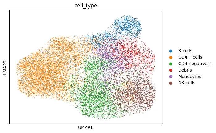
Names instead of numbers is the whole difference. Eight clusters carry six labels, because two of them are CD4 T cells and two are CD4 negative T cells, which is what a panel with no CD8 marker can resolve. The B cells sit as a separate island, and the T cell populations meet along a populated boundary rather than a gap, which is what forced the metaclustering step to cut somewhere.
The margins are worth reading against the picture rather than on their own. The largest, 0.509, belongs to a CD4 T cell cluster, and the smallest, 0.129, belongs to the NK cells at the lower right. That NK label is correct: CD3 0.08 with CD7 3.68 and no CD20 is an NK cell. A small margin means two rules scored similarly, not that the winner is wrong.
The label that is wrong
Section titled “The label that is wrong”One label is wrong, and it is not the one with the smallest margin. The cluster in the
upper right is called debris on a margin of 0.331, and its CD45 median is 4.61, which is
high. It only scores as negative because the scaling runs each marker from the lowest
cluster to the highest, so neg means “the lowest of the eight clusters here” rather than
“below the positive population”.
That is the flaw in scoring against scaled medians, and it bites hardest when the rule table names a population the data does not contain. This subsample holds no real debris, so the debris rule went to whichever cluster sat lowest and produced a confident looking margin while doing it. The margin measures how far the best rule beat the second best, not whether the best rule was right at all.
A rule table needs its neg expectations anchored to a control or to a fixed threshold
before those labels stand on their own. Read the medians beside them until they are.
Reading the two results
Section titled “Reading the two results”The marker profiles are the thing to compare, not the labels, and on the same arcsinh scale
they line up. Python’s cluster_0 sits at CD3 3.44, CD4 3.64 and CD7 2.91, which is R’s
metacluster 1 at 3.50, 3.63 and 2.79. Both engines found the same CD4 T cell population and
gave it a different name.
The numbering carries no meaning across the two, and neither does the count on its own. What transfers is the profile.