Neural Networks with PyTorch

Gradient-boosted trees usually win on tabular data. But neural networks matter when you have many samples, want to learn shared representations across tasks, or need to feed the model something trees cannot handle directly, like raw sequences or images.

This page builds a multilayer perceptron (MLP), the simplest neural network, and trains it end to end with PyTorch. The next page uses a convolutional network on sequence data.

Every code block runs on CPU in a container in the companion repository, so the numbers and the loss curve are real.

When to reach for a neural network

Situation	Better choice
A few thousand rows of tabular features	Gradient-boosted trees
Hundreds of thousands of rows	Neural network competitive
Raw sequences, images, spectra	Neural network (CNN, transformer)
Need calibrated probabilities fast	Logistic regression or trees
Multi-task or transfer learning	Neural network

Do not default to deep learning on small tabular datasets. Start with the tree pages, then reach here when the data justifies it.

The building blocks

A PyTorch model has three pieces: a module that defines the layers, a loss function, and an optimizer that updates the weights.

import torch
import torch.nn as nn

torch.manual_seed(42)


class MLP(nn.Module):
    def __init__(self, n_features):
        super().__init__()
        self.net = nn.Sequential(
            nn.Linear(n_features, 64), nn.ReLU(), nn.Dropout(0.3),
            nn.Linear(64, 32), nn.ReLU(),
            nn.Linear(32, 1))

    def forward(self, x):
        return self.net(x)

• nn.Linear(in, out) is a fully connected layer: out = x @ W + b.
• nn.ReLU() is the nonlinearity. Without it, stacked linear layers collapse into one.
• nn.Dropout(0.3) randomly zeroes 30% of activations during training to reduce overfitting. It is disabled automatically at evaluation time.
• The final layer outputs a single number (the logit). We apply the sigmoid later.

Prepare the data as tensors

Neural networks need scaled inputs and float32 tensors. We use a train, validation, and test split: train fits the weights, validation watches for overfitting, test gives the final estimate.

X = StandardScaler().fit_transform(X)
Xtr = torch.tensor(X_tr, dtype=torch.float32)
ytr = torch.tensor(y_tr, dtype=torch.float32).unsqueeze(1)

Always scale inputs for neural networks

Unlike trees, neural networks are sensitive to feature scale. Fit the StandardScaler on the training split only, then apply it to validation and test, exactly as on the preprocessing page.

The training loop

Each epoch: zero the gradients, forward pass, compute loss, backpropagate, step the optimizer. We track the loss on the validation set to watch for overfitting.

model = MLP(X.shape[1])
optimizer = torch.optim.Adam(model.parameters(), lr=1e-3)
criterion = nn.BCEWithLogitsLoss()

for epoch in range(1, 101):
    model.train()
    optimizer.zero_grad()
    loss = criterion(model(Xtr), ytr)
    loss.backward()
    optimizer.step()

    model.eval()
    with torch.no_grad():
        vloss = criterion(model(Xval), yval).item()

Epoch  20: train loss 0.6190, val loss 0.6230
Epoch  40: train loss 0.4900, val loss 0.4989
Epoch  60: train loss 0.3267, val loss 0.3816
Epoch  80: train loss 0.2284, val loss 0.2916
Epoch 100: train loss 0.1728, val loss 0.2366

BCEWithLogitsLoss combines a sigmoid and binary cross-entropy in one numerically stable step, so the model outputs raw logits and the loss handles the rest.

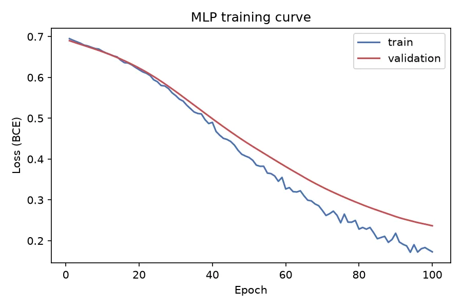
Both curves fall together and the validation loss keeps dropping, so the model is still learning and not yet overfitting. If the validation curve turned upward while the training curve kept falling, that gap would signal overfitting: the moment to stop (early stopping) or add regularization.

Evaluate on the test set

At evaluation, put the model in eval() mode (which disables dropout) and apply the sigmoid to turn logits into probabilities.

model.eval()
with torch.no_grad():
    prob = torch.sigmoid(model(Xte)).numpy().ravel()

print("Test accuracy:", accuracy_score(y_test, (prob > 0.5).astype(int)))
print("Test ROC-AUC: ", roc_auc_score(y_test, prob))

Test accuracy: 0.9033
Test ROC-AUC:  0.9674

A solid result on this synthetic dataset. Compare it against a gradient-boosted tree on the same data before concluding the network is worth the extra complexity.

Key concepts

Concept	What it does
nn.Module	Container for layers and the forward pass
Optimizer (Adam)	Updates weights from gradients
Loss (BCEWithLogitsLoss)	Measures error, drives the gradients
loss.backward()	Backpropagation: computes gradients
optimizer.step()	Applies one weight update
model.train() / eval()	Toggles dropout and batch-norm behavior
torch.no_grad()	Skips gradient tracking for faster inference

Practical tips

• Batch your data with DataLoader once it does not fit in memory. Here the dataset is small enough to train full-batch.
• Watch the validation loss. Stop when it stops improving.
• Tune the learning rate first. It matters more than the architecture.
• Add a GPU by moving the model and tensors with .to("cuda"). Everything here runs on CPU because the dataset is small.

Summary

The MLP is the foundation. A model class, a loss, an optimizer, and a loop that repeats forward, backward, step. The next page keeps the same loop and swaps the architecture for a convolutional network that reads biological sequences.