Count Regression, Poisson & Negative Binomial

The question

Sequencing 120 tumours, does the treated arm carry more somatic variants than the control arm? The outcome is a count, so the answer is a rate ratio, not a difference in means, and the samples were not sequenced to equal depth, so the model has to account for that before it can say anything about biology.

Every code block on this page runs in a container in the companion repository. The numbers and figure come from those real runs.

When to use it, and when not to

Reach for count regression whenever the outcome is a non-negative integer produced by counting things: variants per sample, reads per gene, colonies per plate, cells per field, adverse events per patient-year.

Start with Poisson. It assumes the variance equals the mean, and when that holds it is the most efficient choice. Then check it, because in biology it usually does not hold. When the variance exceeds the mean, move to the negative binomial, which adds a dispersion parameter and widens the intervals accordingly.

Do not run a t-test on counts that are small or skewed, and do not log-transform to force normality when the counts include zeros: log(0) is undefined and log(x + 1) distorts the low end where most of the data often sits. Use a model built for counts.

The data

variant_counts.csv has 120 tumour samples, 60 control and 60 treated, each with a somatic variant count and a sequencing coverage. Coverage varies about threefold across the cohort, independently of arm, which matters: a deeper sample finds more variants for no biological reason at all.

The counts are generated from a negative binomial with theta = 4, so this fixture has a known right answer. A Poisson fit is wrong here in a specific, measurable way, and the point of the page is to measure it rather than assert it.

Assumptions and how to check them

Poisson makes one strong assumption: variance equals mean. The check is the Pearson chi-squared statistic divided by the residual degrees of freedom. Near 1 is fine. Well above 1 is overdispersion, and it means every standard error the model printed is too small.

On this data that ratio is 8.17. The variance is eight times the mean, so the Poisson fit is not close.

There is a second thing to get right, and it is not an assumption so much as a modelling decision. Coverage belongs in the model as an offset, not as an ordinary predictor. An offset asserts that doubling the depth doubles the expected count: its coefficient is fixed at 1 rather than estimated. That is what makes the result a rate per unit coverage rather than a raw count.

library(MASS)   # glm.nb; MASS ships with R

df <- read.csv("variant_counts.csv")
df$arm <- factor(df$arm, levels = c("control", "treated"))

# Poisson, with coverage as an offset.
pois <- glm(n_variants ~ arm + offset(log(coverage)), family = poisson,
  data = df)

# The overdispersion check.
disp <- sum(residuals(pois, type = "pearson")^2) / df.residual(pois)

# Negative binomial: same model, one extra parameter.
nb <- glm.nb(n_variants ~ arm + offset(log(coverage)), data = df)

summary(nb)
c(dispersion = disp, theta = nb$theta)

import numpy as np, pandas as pd
import statsmodels.api as sm
import statsmodels.formula.api as smf

df = pd.read_csv("variant_counts.csv")
df["arm"] = pd.Categorical(df["arm"], categories=["control", "treated"])
offset = np.log(df["coverage"].to_numpy())

# Poisson, with coverage as an offset.
pois = smf.glm("n_variants ~ arm",
               data=df,
               family=sm.families.Poisson(),
               offset=offset).fit()

# The overdispersion check.
disp = float((pois.resid_pearson**2).sum()) / pois.df_resid

# Negative binomial. statsmodels estimates the dispersion as alpha; R reports
# theta = 1 / alpha, so convert before comparing the two.
nb = smf.negativebinomial("n_variants ~ arm", data=df,
                          offset=offset).fit(disp=0)
theta = 1.0 / float(nb.params["alpha"])

print(nb.summary(), disp, theta)

Reading the output

The two models agree almost exactly on the effect and disagree completely on the uncertainty.

	log rate ratio	standard error	p
Poisson	0.4340	0.0407	1.4e-26
Negative binomial	0.4352	0.1026	2.2e-05

The point estimate barely moves, 0.4340 to 0.4352, because Poisson coefficients stay consistent under overdispersion. What changes is the standard error, which is 2.52 times wider once the dispersion is modelled. The Poisson p-value of 1.4e-26 is not a stronger result. It is the same result with the uncertainty removed.

Report the rate ratio, not the log: exp(0.4352) = 1.545, 95% CI 1.264 to 1.889. Treated samples carry about 55% more variants per unit coverage.

The estimated theta is 3.80, against the 4 the data was generated with. AIC drops from 1404.1 to 900.0, which is not a close call.

Visualizing it

Bin the samples by fitted rate and plot the observed variance in each bin against what each model predicts. Poisson’s assumption is the diagonal line, variance equals mean. The negative binomial curve is mean + mean squared over theta.

R
Python

Observed variance per bin sitting far above the Poisson line and close to the negative binomial curve (R)

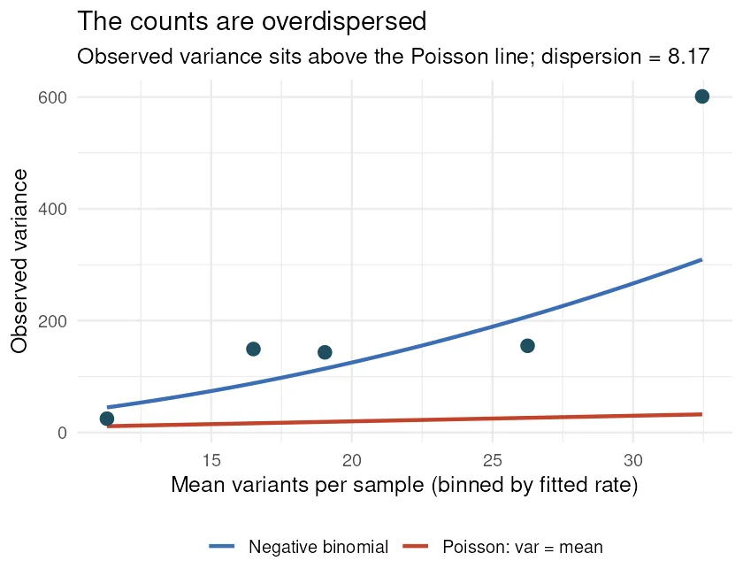
Every point sits far above the red line. This figure is worth drawing before you trust any count model, and it takes four lines.

Pitfalls and bioinformatics notes

The dispersion check is not optional. Poisson never warns you. It returns a clean-looking table with impossibly small standard errors, and nothing in the output says the assumption failed.
An offset is not a covariate. Putting coverage on the right-hand side as an ordinary predictor estimates a coefficient for it, which answers a different question. If you believe depth scales the count proportionally, say so with an offset and let the model spend its degrees of freedom elsewhere.
This is why RNA-seq tools use the negative binomial. DESeq2 and edgeR both model counts this way, and both spend most of their machinery on estimating dispersion well from few replicates. The problem on this page is the same problem at genome scale.
Quasi-Poisson is the other option. It inflates the standard errors by a dispersion factor without a full likelihood. It is fine for testing, but it gives no AIC and no generative model, so the negative binomial is usually the better default.
A linear model on counts is not automatically absurd. The textbook objection is that it predicts negatives, and on this fixture it does not: its smallest fitted value is 4.90. The real failure here is constant variance, which the figure above disproves directly. Check the actual failure rather than reciting the usual one.

Key points

Counts need a count model. The output is a rate ratio.
Fit Poisson, then immediately check Pearson chi-squared over residual df.
Overdispersion leaves the estimate alone and destroys the standard error. Here the SE was 2.52 times too small and the p-value 21 orders of magnitude too confident.
Exposure differences belong in an offset, with a fixed coefficient of 1.
Negative binomial adds theta and converges on Poisson as theta grows.