CNNs for Sequences with PyTorch

Trees and MLPs need a fixed table of features. Biological sequences are different: a motif can appear at any position, and what matters is the local pattern, not the absolute coordinate. Convolutional networks are built for exactly this. A convolutional filter slides along the sequence and fires wherever it sees its pattern, so the same motif is detected no matter where it sits.

This page trains a 1D CNN to tell apart DNA sequences that carry a transcription-factor motif from those that do not, then reads the learned filter back out as a motif. It builds directly on the MLP page: same training loop, different architecture.

Everything runs on CPU in a container in the companion repository.

The task: detect a planted motif

We generate 2000 sequences of 200 base pairs. Positive sequences carry the AP-1 motif TGACGTCA (with up to one point mutation) inserted at a random position; negative sequences are random. This mimics detecting a binding site in a promoter.

NT = np.array(list("ACGT"))
MOTIF = np.array([3, 2, 0, 1, 2, 3, 1, 0])  # TGACGTCA, encoded A=0 C=1 G=2 T=3

seqs = rng.integers(0, 4, size=(N, L))
for i in range(N):
    if y[i] == 1:
        pos = rng.integers(0, L - 8)
        seqs[i, pos:pos + 8] = MOTIF   # (with an optional single mutation)

Sequences: 2000 x 200 bp, positives: 1030 negatives: 970

One-hot encoding

A CNN reads sequences as a (4, L) matrix: four channels (A, C, G, T), each a binary track along the sequence. The batch shape is (N, 4, L).

onehot = np.eye(4, dtype=np.float32)[seqs].transpose(0, 2, 1)  # (N, 4, L)
X = torch.tensor(onehot)

The convolutional network

One convolutional layer scans for motifs. Global max-pooling reports the single strongest hit anywhere in the sequence, which is exactly the “is the motif present?” question. A linear layer turns the 16 filter responses into one logit.

class SeqCNN(nn.Module):
    def __init__(self):
        super().__init__()
        self.conv = nn.Conv1d(4, 16, kernel_size=8)   # 16 filters, 8 bp wide
        self.pool = nn.AdaptiveMaxPool1d(1)           # strongest hit per filter
        self.fc = nn.Linear(16, 1)

    def forward(self, x):
        h = torch.relu(self.conv(x))
        h = self.pool(h).squeeze(-1)
        return self.fc(h)

• Conv1d(4, 16, kernel_size=8) learns 16 filters, each 8 bp wide, matching the motif length. Each filter is effectively a learnable position weight matrix.
• AdaptiveMaxPool1d(1) makes the model position-invariant: it keeps only the maximum response, so a motif at position 12 and one at position 180 look the same.

Mini-batch training

Unlike the full-batch MLP, we train in mini-batches. Each batch is one gradient step, so an epoch gives many updates and the network converges in a handful of epochs.

optimizer = torch.optim.Adam(model.parameters(), lr=5e-3)
criterion = nn.BCEWithLogitsLoss()

for epoch in range(1, 31):
    model.train()
    perm = torch.randperm(n_tr, generator=g)
    for i in range(0, n_tr, 64):
        idx = perm[i:i + 64]
        optimizer.zero_grad()
        loss = criterion(model(Xtr[idx]), ytr[idx])
        loss.backward()
        optimizer.step()

Epoch  5: train loss 0.6339
Epoch 10: train loss 0.2568
Epoch 15: train loss 0.1877
Epoch 20: train loss 0.1613
Epoch 25: train loss 0.1460
Epoch 30: train loss 0.1299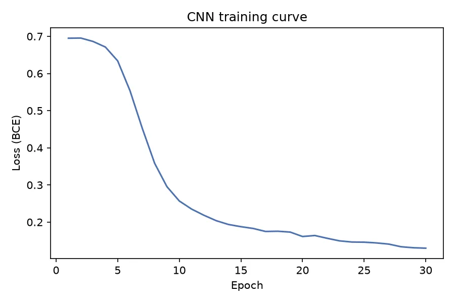

The loss sits flat for a few epochs while the random filters drift, then drops sharply once a filter locks onto the motif.

Full-batch training stalls here

With one gradient step per epoch (as on the MLP page) this CNN barely moves. Mini-batches give tens of updates per epoch, which is what lets it converge. Batch size and learning rate matter more for CNNs than the exact architecture.

Evaluate

model.eval()
with torch.no_grad():
    prob = torch.sigmoid(model(Xte)).numpy().ravel()

print("Test accuracy:", accuracy_score(yte, (prob > 0.5).astype(int)))
print("Test ROC-AUC: ", roc_auc_score(yte, prob))

Test accuracy: 0.9167
Test ROC-AUC:  0.9790

The network detects the motif almost perfectly, and it never saw the motif’s identity or location. It learned both from labels alone.

Reading the motif back out of the filters

The best part: a trained filter is a motif detector, so we can recover the biology. We run the convolution over every sequence, pick the filter that best separates positives from negatives, and collect the 8 bp windows where it fires hardest. Stacking those windows into a position frequency matrix reconstructs the motif.

sep = acts[pos].max(2).mean(0) - acts[neg].max(2).mean(0)   # per-filter separation
best = sep.argmax()
windows = [seqs[i, acts[i, best].argmax():acts[i, best].argmax() + 8]
           for i in positives]
pwm = np.stack([(windows == nt).mean(0) for nt in range(4)])

Planted motif:   TGACGTCA
Recovered motif: GACGTCAC  (filter #0)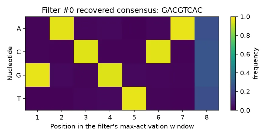

The recovered consensus is the GACGTCA core of the AP-1 motif. The filter latched onto the motif offset by one base, so its 8 bp window captures the last seven motif bases plus one random flanking base (the diffuse final column). The network was never told the motif; it discovered it from the classification signal alone. This is how tools like DeepBind and Basset turn learned filters back into interpretable sequence logos.

When to use a CNN

Data	Model
Fixed tabular features	Trees or MLP
DNA / RNA / protein sequences	1D CNN
Images, spatial data	2D CNN
Long-range dependencies in sequence	CNN + attention, or a transformer

Summary

The CNN kept the MLP’s training loop and swapped in a convolution that scans for local patterns anywhere in the input. It learned to detect a DNA motif from labels alone, and its filters could be read back as the motif itself. That combination, position invariance plus interpretable filters, is why CNNs became a workhorse for regulatory genomics.