qPCR Files

A qPCR instrument measures fluorescence in every well at every cycle. The raw record of a run is therefore a matrix of amplification curves, and the summary everyone quotes is the Cq, the cycle at which each curve crosses a threshold. The files arrive in two families. RDML is the vendor-independent interchange standard, and each vendor’s software also writes its own export tables.

RDML: the interchange standard

RDML, the Real-time PCR Data Markup Language, is an XML schema maintained at rdml.org, designed so a run from one vendor’s instrument can be analysed in another vendor’s software. On disk an .rdml file is a zip archive holding one XML document. The RDML package on Bioconductor reads it, and ships example files written by three different vendors’ instruments. The first one comes from an Applied Biosystems StepOne.

library(RDML)

rdml_file <- system.file("extdata", "stepone_std.rdml", package = "RDML")
file.size(rdml_file)

# An RDML file on disk is a zip archive holding one XML document.
unzip(rdml_file, list = TRUE)

# The XML inside: samples with their types, then per-well data points.
inner_lines <- readLines(unz(rdml_file, "rdml_data.xml"), n = 25)
cat(inner_lines, sep = "\n")

[1] 8740
           Name Length                Date
1 rdml_data.xml 148636 2014-09-05 12:29:00
<?xml version="1.0" encoding="UTF-8" standalone="yes"?>
<rdml xmlns="http://www.rdml.org" version="1.0">
    <dateMade>2014-09-05T00:29:23.361</dateMade>
    <dateUpdated>2014-09-05T00:29:23.361</dateUpdated>
    <sample id="NTC_RNase P">
        <type>ntc</type>
    </sample>
    <sample id="pop1_RNase P">
        <type>unkn</type>
    </sample>
    <sample id="pop2_RNase P">
        <type>unkn</type>
    </sample>
    <sample id="STD_RNase P_10000.0">
        <type>std</type>
        <quantity>
            <value>10000.0</value>
            <unit>other</unit>
        </quantity>
    </sample>
    <sample id="STD_RNase P_5000.0">
        <type>std</type>
        <quantity>
            <value>5000.0</value>
            <unit>other</unit>

The XML declares the samples and their types. This experiment is a standard curve: ntc wells carry no template, unkn wells are the unknowns, and std wells carry known input quantities of the RNase P amplicon. Further down the document, one react element per well holds the data points, cycle number and fluorescence, plus the Cq the instrument software calculated.

Three vendors, one standard

The RDML package bundles example files from three vendors: the StepOne file, a Bio-Rad CFX96 run with a melt curve, and a Roche LightCycler 96 run. One reader handles all three, which is the point of the standard.

rdml_examples <- c(
  stepone = system.file("extdata", "stepone_std.rdml", package = "RDML"),
  biorad = system.file("extdata", "BioRad_qPCR_melt.rdml", package = "RDML"),
  lightcycler = system.file("extdata", "lc96_bACTXY.rdml", package = "RDML")
)

summaries <- lapply(rdml_examples, function(path) {
  # RDML$new() prints progress to stdout; capture it so only the table shows.
  invisible(capture.output(rdml <- RDML$new(path)))
  fdata <- rdml$GetFData(long.table = TRUE)
  data.frame(
    wells = length(unique(fdata$fdata.name)),
    runs = length(unique(fdata$run.id)),
    targets = length(unique(fdata$target)),
    has_melt_data = any(fdata$mdp, na.rm = TRUE),
    stringsAsFactors = FALSE
  )
})
do.call(rbind, summaries)

            wells runs targets has_melt_data
stepone        24    1       1         FALSE
biorad         60    1       4          TRUE
lightcycler    64    1       4         FALSE

The three files differ in size and content but unpack to the same long table: one row per well per cycle, with the sample, target, dye and fluorescence. The Bio-Rad file also carries melt data points, the fluorescence trace recorded while the temperature rises after amplification.

The amplification curves

The amplification curve is what the file actually records. Here are the standards from the StepOne run, one line per well, coloured by input quantity.

library(ggplot2)

invisible(capture.output(stepone <- RDML$new(rdml_examples[["stepone"]])))
amp_data <- stepone$GetFData(long.table = TRUE)
amp_data <- amp_data[!is.na(amp_data$fluor), ]

# Keep the standards and recover the input quantity from the sample name.
std_data <- amp_data[grepl("^STD", amp_data$sample), ]
std_data$quantity <- as.numeric(sub("STD_RNase P_", "", std_data$sample))

curve_plot <- ggplot(std_data,
                     aes(x = cyc, y = fluor, group = fdata.name,
                         colour = factor(quantity))) +
  geom_line(alpha = 0.7) +
  labs(x = "Cycle", y = "Fluorescence", colour = "Input copies")

dir.create("outputs", showWarnings = FALSE, recursive = TRUE)
ggsave("outputs/qpcr_amplification_curves.png", plot = curve_plot,
       width = 7, height = 4, dpi = 110, bg = "white")

# The table behind the plot.
head(as.data.frame(std_data)[, c("fdata.name", "cyc", "fluor",
                                 "sample.type")], 4)

                           fdata.name cyc     fluor sample.type
1 B02_STD_RNase P_10000.0_std_RNase P   1 0.6265384         std
2 B02_STD_RNase P_10000.0_std_RNase P   2 0.6273690         std
3 B02_STD_RNase P_10000.0_std_RNase P   3 0.6276071         std
4 B02_STD_RNase P_10000.0_std_RNase P   4 0.6288173         std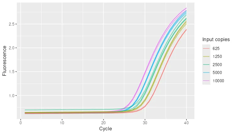

Amplification curves for the fifteen standard wells of the StepOne run. Each line is one well, coloured by input quantity from 625 to 10000 copies. The curves shift left as the input increases, so the highest input crosses the threshold first.

More input means fewer cycles to reach the threshold, so the curves order themselves by quantity from right to left.

The Cq values and the standard curve

The Cq values the instrument calculated sit in the XML, one per well, inside the react elements. The package does not surface them directly, so the code below pulls them out with xml2, which RDML itself uses, and joins them with the plate layout.

library(xml2)

doc <- read_xml(unz(rdml_examples[["stepone"]], "rdml_data.xml"))
ns <- c(rdml = "http://www.rdml.org")
reacts <- xml_find_all(doc, "//rdml:react", ns)

cq_table <- data.frame(
  position = xml_attr(reacts, "id"),
  cq = as.numeric(xml_text(xml_find_first(reacts, ".//rdml:cq", ns))),
  stringsAsFactors = FALSE
)

# Attach the sample metadata the package already parsed.
plate_map <- as.data.frame(stepone$AsTable())[, c("position", "sample",
                                                  "sample.type")]
plate_map$position <- sub("^(.)0", "\\1", plate_map$position)
cq_table <- merge(cq_table, plate_map, by = "position")

# The standards carry the input quantity in the sample name.
std_cq <- cq_table[cq_table$sample.type == "std", ]
std_cq$quantity <- as.numeric(sub("STD_RNase P_", "", std_cq$sample))

# Cq falls linearly with the log of the input. The slope gives the efficiency.
fit <- lm(cq ~ log10(quantity), data = std_cq)
coef(fit)
efficiency <- 10^(-1 / coef(fit)[2]) - 1
cat("amplification efficiency:", round(efficiency * 100, 1), "%\n")

    (Intercept) log10(quantity)
      40.768072       -3.477042
amplification efficiency: 93.9 %

A perfect assay doubles the product every cycle, which gives a slope of -3.32 and an efficiency of 100 percent. This teaching file lands at 93.9 percent. The no-template controls report a Cq of 40, which is the software’s way of saying the reaction never crossed the threshold within the run.

std_plot <- ggplot(std_cq, aes(x = quantity, y = cq)) +
  geom_point(size = 2) +
  scale_x_log10() +
  geom_smooth(method = "lm", se = FALSE, colour = "grey30") +
  labs(x = "Input copies (log scale)", y = "Cq")

ggsave("outputs/qpcr_standard_curve.png", plot = std_plot,
       width = 6, height = 4, dpi = 110, bg = "white")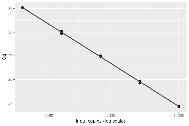

The standard curve: Cq against input copies on a log scale for the fifteen standard wells. The points fall on a straight line, because each tenfold increase in input needs the same number of fewer cycles.

Vendor export tables

RDML is the interchange format, but the file that lands in your inbox is usually the vendor software’s own export table, and every vendor lays it out differently. Bio-Rad’s CFX Manager writes a comma-separated results table with one row per well per target, and leaves the Cq empty for the no-template controls.

library(readr)

# Bio-Rad CFX Manager: a comma-separated results table.
cfx <- read_csv("/opt/data/biorad_cfx_export.csv", show_col_types = FALSE)
head(cfx, 4)

# QuantStudio: tab-delimited, with a preamble before the [Results] section.
raw_lines <- readLines("/opt/data/quantstudio_export.tsv")
table_start <- grep("^\\[Results\\]$", raw_lines)
cat("results table starts at line", table_start, "\n")

quantstudio <- read.delim("/opt/data/quantstudio_export.tsv",
                          skip = table_start)
head(quantstudio[, c("Well.Position", "Sample.Name", "Target.Name", "CT")], 4)
cat("undetermined CT values:", sum(quantstudio$CT == "Undetermined"), "\n")

# A tibble: 4 × 7
  Well  Fluor Target Content Sample     Cq `Starting Quantity (SQ)`
  <chr> <chr> <chr>  <chr>   <chr>   <dbl> <lgl>
1 A01   SYBR  Actb   Unkn    Liver_1  21.7 NA
2 B01   SYBR  Gapdh  Unkn    Liver_1  24   NA
3 C01   SYBR  Il6    Unkn    Liver_1  29.9 NA
4 D01   SYBR  Actb   Unkn    Liver_2  22.2 NA
results table starts at line 7
  Well.Position Sample.Name Target.Name    CT
1           A01     Liver_1        Actb 22.37
2           B01     Liver_1         Il6 30.08
3           C01     Liver_2        Actb 22.47
4           D01     Liver_2         Il6 30.14
undetermined CT values: 2

Two details of the QuantStudio export matter in practice. The table does not start at line one, so you locate the [Results] marker before reading. And a well that never amplified carries the text Undetermined in the CT column, which turns the column into text when you read it. Convert it to numeric after reading and the undetermined wells become missing values, which is what they are.

These two files are synthetic fixtures that imitate the export layouts. Real exports add more columns, and the exact set changes between software versions, so always check the column names of a new export before you trust a parser.

The proprietary containers

Both vendors also write native run files. QuantStudio’s .eds is a zip archive of internal tables, and Roche’s LightCycler .ixo is a proprietary binary. Neither is meant to be parsed directly. The supported route out of them is the vendor software’s own export, either to a results table or to RDML, and RDML is the format to ask for when the data will be analysed away from the instrument.

Summary

A qPCR run is a matrix of amplification curves, one per well, plus a Cq per well.
RDML is the vendor-independent standard: a zip archive holding one XML document, readable with the RDML package.
The example files bundled with the package come from StepOne, Bio-Rad CFX96 and LightCycler 96 instruments, and one reader handles all three.
Vendor export tables differ in layout. QuantStudio puts the table after a preamble, and encodes failed wells as the text Undetermined.
The standard curve relates Cq to log input, and its slope estimates the amplification efficiency.