Repertoire Analysis

After preprocessing and quality filtering, the real analysis begins. BCR repertoire analysis answers questions about which antibodies are present, how diverse the repertoire is and whether specific clones have expanded in response to antigen.

V(D)J assignment

The first analysis step is V(D)J assignment. Each antibody sequence must be mapped back to the germline V, D and J gene segments that were used in its recombination.

IgBLAST is the standard tool for this task. It aligns each sequence against the IMGT reference database of germline gene segments. The output tells you:

• Which V gene was used (for example IGHV3-30)
• Which D gene was used (for example IGHD3-10)
• Which J gene was used (for example IGHJ4)
• The CDR3 nucleotide and amino acid sequence
• The number of mutations relative to the germline V gene

IgBLAST uses the IMGT numbering scheme to define framework and CDR regions consistently across all sequences. This standardisation is critical for comparing results across studies.

Tip

Always use the latest IMGT reference database. Gene nomenclature and allele definitions are updated regularly. An outdated reference can cause incorrect V gene assignments.

V gene usage

V gene usage analysis counts how often each V gene appears in the repertoire. This reveals biases in the immune response.

In a healthy human, the IGHV3 family dominates the heavy chain repertoire. IGHV1 and IGHV4 are the next most common. The distribution is not uniform. Some V genes are used far more often than others due to differences in recombination efficiency and selection.

V gene usage shifts in disease:

• IGHV4-34 is expanded in systemic lupus erythematosus (SLE). This V gene encodes antibodies that bind self-antigens.
• IGHV1-69 is enriched in responses to influenza and hepatitis C virus. Its germline-encoded CDR2 binds the haemagglutinin stem.
• IGHV3-30 and IGHV3-33 are common in COVID-19 responses targeting the spike protein.

V gene usage is typically visualised as a bar chart showing the frequency of each V gene across samples or conditions. The chart below counts sequences per germline IGHV gene in one AIRR-format table, the kind of file airrflow writes into changeo/, committed beside this page’s code in the companion repository. The IGHV3 family occupies the top ranks, and the spread between genes is wide: that unevenness is what primer bias, recombination efficiency and selection each contribute to.

library(immunarch)
library(ggplot2)

# One AIRR table as airrflow writes it into changeo/.
imm <- repLoad("sample01_airr.tsv")

# Sequences per germline V gene.
gu <- geneUsage(imm$data, .gene = "hs.ighv")
ggsave(
  "outputs/vgene-usage.png",
  vis(gu),
  width = 7.5, height = 4.5, dpi = 130, bg = "white"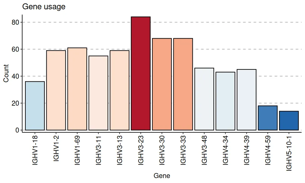
)

CDR3 analysis

The CDR3 region is the most variable part of the antibody. It is formed by the junction of V, D and J segments, with random nucleotide additions and deletions at the joins. CDR3 makes the most contacts with antigen and largely determines binding specificity.

Key CDR3 properties to analyse:

• Length distribution: CDR3 length is measured in amino acids. The average heavy chain CDR3 is about 15 amino acids. IgG CDR3 tends to be shorter than IgM CDR3 because antigen selection favours certain lengths.
• Amino acid composition: hydrophobicity, charge and aromaticity of the CDR3 sequence. Broadly neutralising antibodies against HIV tend to have long, hydrophobic CDR3 loops.
• Sequence motifs: recurrent CDR3 sequences shared across individuals (public clonotypes) can indicate convergent immune responses to common pathogens.

CDR3 length distributions are usually shown as histograms, often split by isotype to highlight differences between IgM and class-switched antibodies. immunarch calls this a spectratype; on the toy table it lands where heavy-chain CDR3s land, with the peak at thirteen and fourteen residues:

# CDR3 amino acid length distribution.
sp <- spectratype(imm$data[[1]], .col = "aa")
ggsave(
  "outputs/cdr3-lengths.png",
  vis(sp),
  width = 7, height = 4, dpi = 130, bg = "white"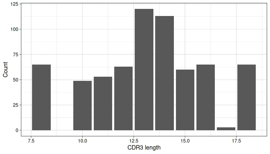
)

Isotype distribution

Isotype analysis reveals the functional state of the B cell compartment. Each isotype has a different effector function.

Isotype	Function	Typical context
IgM	First responder, low affinity	Early immune response, naive B cells
IgD	Co-expressed with IgM on naive cells	Rarely sequenced, low abundance
IgG	High-affinity, systemic immunity	Secondary responses, vaccination
IgA	Mucosal immunity	Gut, respiratory tract
IgE	Allergy and anti-parasite	Allergic responses, helminth infections

Isotype distribution changes with immune activation. A resting repertoire is dominated by IgM. After vaccination or infection, the IgG and IgA fractions increase as B cells undergo class switching.

In BCR sequencing data, isotype is determined by the constant region primer or by aligning the constant region sequence. The ratio of IgG to IgM is a simple but informative metric of immune activation.

Somatic hypermutation analysis

Somatic hypermutation (SHM) introduces point mutations into the variable region after a B cell encounters antigen. Cells with improved binding are selected and expanded. This is affinity maturation.

SHM analysis measures:

• Mutation frequency: the percentage of nucleotides that differ from the germline V gene. A naive B cell has near-zero mutations. A highly mutated memory B cell may have 5 to 15% mutation frequency.
• Replacement vs silent mutations: replacement mutations change the amino acid. Silent mutations do not. Antigen-driven selection favours replacement mutations in CDRs because these affect binding. A high ratio of replacement to silent mutations in CDRs is evidence of positive selection.
• CDR vs framework mutations: mutations in CDRs are more likely to affect binding. Mutations in framework regions are more likely to destabilise the antibody structure. Selection tends to accumulate replacement mutations in CDRs while keeping framework regions conserved.

The BASELINe method quantifies selection by comparing the observed pattern of replacement and silent mutations to what would be expected by chance. A positive selection score in CDRs indicates antigen-driven selection.

Note

SHM analysis requires accurate germline V gene assignment. If IgBLAST assigns the wrong germline allele, the mutation count will be inflated or deflated. Using personalised germline databases (for example from TIgGER) improves accuracy.

Clonal analysis

B cells descended from the same V(D)J recombination event form a clone. Within a clone, somatic hypermutation creates a family of related sequences with slightly different mutations. These are called clonal families or lineage trees.

Defining clones

Clones are defined by three criteria:

1. Same V gene
2. Same J gene
3. Similar CDR3 sequence (typically above 85% nucleotide identity)

The CDR3 similarity threshold is critical. Too stringent and you split real clones. Too lenient and you merge unrelated sequences. The Immcantation framework uses a data-driven approach: it fits a Gaussian mixture model to the distribution of nearest-neighbour CDR3 distances to find the threshold that separates clonal from non-clonal pairs.

Clonal expansion

Clonal expansion occurs when antigen-driven B cells proliferate. In sequencing data, expanded clones appear as groups of many related sequences.

Key metrics:

• Clone size distribution: most clones contain a single sequence. A few clones contain many sequences. Plot as a rank-abundance curve.
• Top clone fraction: the percentage of the repertoire occupied by the largest clone. Values above 5 to 10% indicate strong expansion.
• Gini index: measures inequality in clone sizes. A value near 0 means all clones are equal size. A value near 1 means the repertoire is dominated by a few clones.

Clonal expansion is expected after vaccination, during active infection and in B cell malignancies. In chronic lymphocytic leukaemia (CLL), a single malignant clone can dominate the entire repertoire.

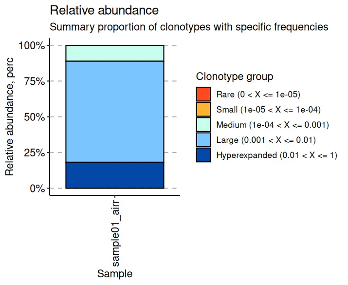
Two plots carry this section. The rank-abundance curve sorts clones by size and shows how quickly the frequency falls; the clonal-space plot asks what share of the repertoire each size class holds. On the toy table, four expanded clone families sit far to the left of roughly six hundred singletons:

# Rank-abundance curve: clone frequency against clone rank.
abundance <- data.frame(
  rank = seq_len(nrow(imm$data[[1]])),
  proportion = sort(imm$data[[1]]$Proportion, decreasing = TRUE)
)
p <- ggplot(abundance, aes(rank, proportion)) +
  geom_line() +
  geom_point(size = 0.4) +
  scale_x_log10() +
  scale_y_log10() +
  labs(x = "Clone rank", y = "Clone frequency")
ggsave(
  "outputs/rank-abundance.png",
  p,
  width = 7, height = 4.5, dpi = 130, bg = "white"
)

# Repertoire space held by each clone-size class.
cs <- repClonality(imm$data, .method = "homeo")
ggsave(
  "outputs/clonal-space.png",
  vis(cs),
  width = 5.5, height = 4.5, dpi = 130, bg = "white"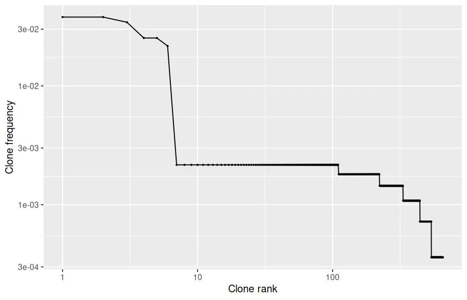
)

Lineage trees

Within an expanded clone, you can reconstruct the lineage tree showing how different sequences evolved from a common ancestor through somatic hypermutation. The unmutated common ancestor (UCA) is inferred by reverting all mutations to germline.

Lineage trees reveal:

• The order in which mutations were acquired
• Whether multiple branches independently acquired the same mutation (convergent evolution)
• The breadth of diversity within a clone

IgPhyML builds these trees with maximum likelihood under a B-cell-specific substitution model that counts mutations at the codon level, and dowser drives it from R and draws the result. The synthetic fixture cannot teach this part, because its sequences carry no real evolutionary history, so this example runs on a published dataset instead: ExampleDb, bundled with alakazam, from Laserson & Vigneault et al. (PNAS 2014), a vaccine-response study sampled over time. Clone 3170 has twenty-eight sequences across two isotypes, small enough to read and big enough to show the structure:

library(alakazam)
library(dowser)
library(dplyr)
library(ggplot2)
library(ggtree)

data(ExampleDb, package = "alakazam")

# One clone with both IgG and IgA members, 28 sequences.
sub <- as.data.frame(ExampleDb) |>
  filter(clone_id == 3170)
print(table(sub$c_call))

clones <- formatClones(sub, traits = "c_call", collapse = FALSE)
trees <- getTrees(
  clones,
  build = "igphyml",
  exec = "/usr/local/share/igphyml/src/igphyml",
  nproc = 1
)

# The likelihood model fit for this clone.
params <- as.data.frame(trees$parameters[[1]])
print(params[, c("tree_length", "lhood", "omega_mle")])

# tips = NULL drops dowser's default layer so shape can join colour.
p <- plotTrees(trees, tips = NULL)[[1]] +
  geom_tippoint(aes(color = c_call, shape = c_call), size = 2.5) +
  scale_color_manual(
    values = c(IGHA = "#2CA02C", IGHG = "#FF7F0E"), name = "Isotype"
  ) +
  scale_shape_manual(values = c(IGHA = 16, IGHG = 15), name = "Isotype")
ggsave(
  "outputs/lineage-tree.png",
  p,
  width = 8, height = 6, dpi = 150, bg = "white"
)

IGHA IGHG
  10   18
  tree_length     lhood omega_mle
1      0.8599 -615.9709    0.4878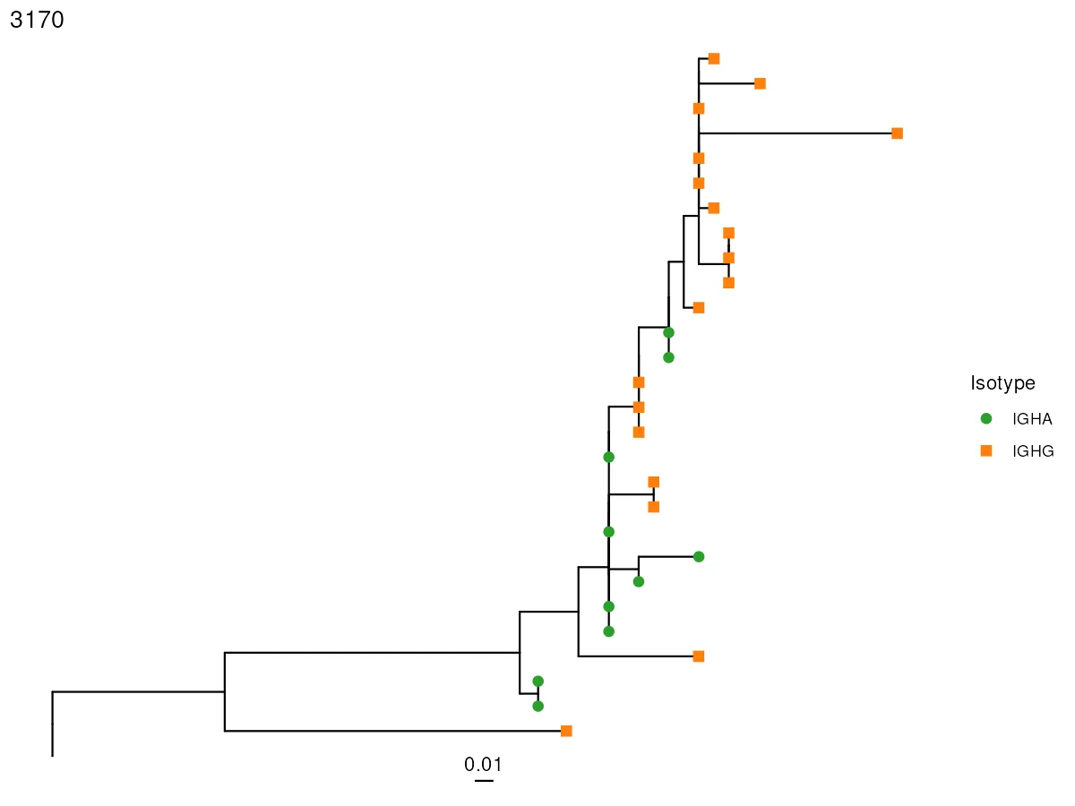

The printed model parameters are worth a look: omega_mle is the fitted dN/dS ratio across the clone, and values below one mark purifying selection, which is the normal background state of a healthy repertoire. The exec path points at the IgPhyML binary inside this site’s container; on your own machine, install it with the Immcantation suite image or compile it from the IgPhyML GitHub release.

Diversity metrics

Repertoire diversity measures how varied the antibody pool is. Higher diversity generally indicates a broader immune capacity.

Common metrics

• Richness (observed clones): the total number of unique clones. Sensitive to sequencing depth. More sequencing finds more clones.
• Shannon index: accounts for both the number of clones and their relative abundance. A repertoire with many equally abundant clones has high Shannon diversity. A repertoire dominated by a few clones has low Shannon diversity.
• Simpson index: the probability that two randomly chosen sequences belong to different clones. Less sensitive to rare clones than Shannon.
• Hill diversity profiles: a family of diversity indices parameterised by a single number q. When q=0 it equals richness, when q=1 the exponential of Shannon, and when q=2 the inverse Simpson. Plotting diversity across q values gives a complete picture.

The Hill profile makes the single-number indices concrete. At q=1 the toy repertoire reads as roughly three hundred and sixty effective clones; as q grows, abundant clones dominate the estimate and the effective count falls below forty:

# Diversity as a function of the order parameter q.
dv <- repDiversity(imm$data, .method = "hill")
ggsave(
  "outputs/hill-diversity.png",
  vis(dv),
  width = 7, height = 4.5, dpi = 130, bg = "white"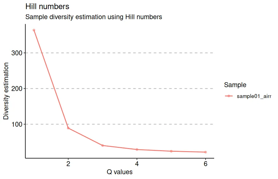
)

Rarefaction

Sequencing depth affects diversity estimates. A sample sequenced more deeply will appear more diverse simply because more rare clones are detected.

Rarefaction curves address this by subsampling to equal depth and recalculating diversity. If the curve has plateaued, you have captured most of the diversity. If it is still rising steeply, deeper sequencing would find more clones.

Always compare diversity between samples at the same rarefied depth.

Tools: the Immcantation framework

The Immcantation suite is the standard toolkit for BCR repertoire analysis. It consists of several packages that work together:

Package	Purpose
pRESTO	Raw read processing, UMI handling, primer masking
Change-O	Parse IgBLAST output, define clones
Alakazam	Diversity analysis, V gene usage, lineage reconstruction
SHazaM	Somatic hypermutation analysis, selection quantification
SCOPer	Spectral clustering for clonal assignment
TIgGER	Infer novel germline alleles from sequencing data
Dowser	Phylogenetic analysis of B cell lineages

A typical workflow:

1. pRESTO: quality filter, UMI consensus, primer masking, paired-end assembly
2. IgBLAST: V(D)J annotation against IMGT reference
3. Change-O: parse annotations, filter non-functional sequences, define clones
4. Alakazam: gene usage plots, diversity analysis, CDR3 properties
5. SHazaM: mutation frequency, selection analysis with BASELINe
6. Dowser: lineage tree reconstruction for expanded clones

All Immcantation tools use the AIRR data format. AIRR-formatted TSV files are the standard interchange format for adaptive immune receptor data.

An Immcantation worked example

Those steps land on this page as alakazam, the Immcantation package for clone-level bookkeeping. Its first analytical job is per-isotype counting through countClones(), the canonical entry point for clone frequencies after assignment. On this page’s committed heavy-chain table the count returns one row per clone with both seq_count and seq_freq:

library(alakazam)
library(dplyr)
library(ggplot2)

sample_df <- read.csv("sample01_airr.tsv", sep = "\t")

# Immcantation's per-isotype clone counting on the AIRR table.
counts <- countClones(sample_df, groups = "c_call")

iso_split <- counts |>
  group_by(c_call) |>
  summarise(sequences = sum(seq_count), .groups = "drop") |>
  mutate(fraction = round(sequences / sum(sequences), 4))
print(as.data.frame(iso_split))

plot_df <- counts
p <- ggplot(plot_df, aes(reorder(c_call, -seq_count), seq_count)) +
  geom_col() +
  labs(x = "Isotype", y = "Sequences")
ggsave(
  "outputs/isotype-clones.png",
  p,
  width = 6, height = 4, dpi = 130, bg = "white"
)

  c_call sequences fraction
1  IGHA1        72   0.1094
2   IGHD        73   0.1109
3   IGHE        89   0.1353
4  IGHG1       132   0.2006
5  IGHG3        75   0.1140
6   IGHM       217   0.3298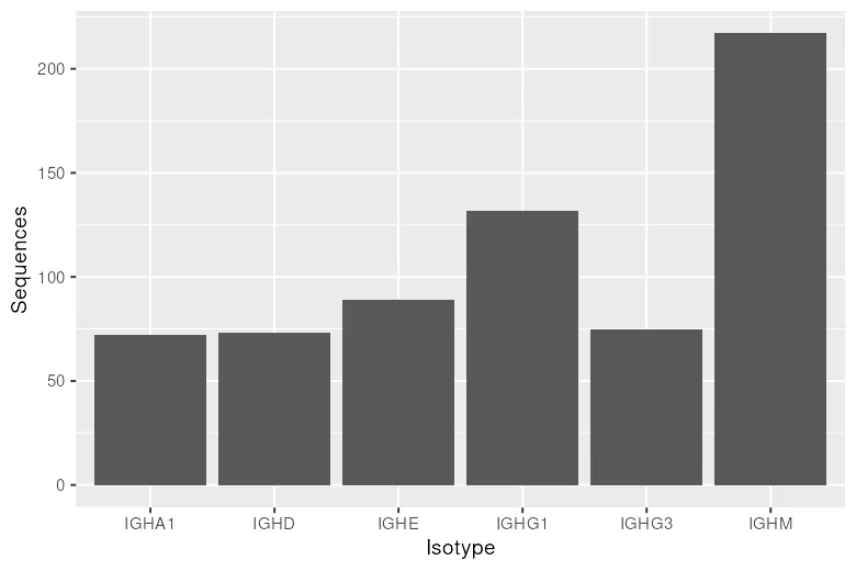

# A clone counts as switched when its members report more than one isotype.
switch_frac <- sample_df |>
  group_by(clone_id) |>
  summarise(isotypes = length(unique(c_call))) |>
  summarise(
    families = n(),
    switched = sum(isotypes > 1),
    fraction = round(mean(isotypes > 1), 3)
  )
print(as.data.frame(switch_frac))

  families switched fraction
1      654        4    0.006

Four of the toy subject’s families carry two to three isotypes, exactly what a class-switching event looks like in annotation data; in real repertoires that distinction is part of how affinity maturation gets quantified. Beyond these single-clone summaries, Alakazam integrates with SHazaM to run BASELINe on the same table, and with Dowser to reconstruct the lineage trees of expanded families; those two live outside this page’s scope because tree reconstruction from partially simulated sequences is a poor teaching target.

Summary

• V(D)J assignment with IgBLAST is the first step. It identifies which germline gene segments were used and counts mutations.
• V gene usage, CDR3 properties and isotype distribution describe the composition of the repertoire.
• Somatic hypermutation analysis reveals affinity maturation and antigen-driven selection.
• Clonal analysis identifies expanded clones and reconstructs their evolutionary history.
• Diversity metrics quantify how broad or focused the repertoire is. Always account for sequencing depth with rarefaction.
• The Immcantation framework provides a complete toolkit from raw reads to biological insight.