Repertoire Analysis
After preprocessing and quality filtering, TCR repertoire analysis answers questions about which T cells are present, how diverse the repertoire is, which clones have expanded and what antigens they might recognise.
V(D)J assignment
Section titled “V(D)J assignment”The first analysis step is V(D)J assignment. Each TCR sequence is mapped back to the germline V, D and J gene segments used in its recombination.
IgBLAST handles this for TCR sequences just as it does for BCR. It aligns each sequence against the IMGT reference database of germline TCR gene segments. The output includes:
- Which V gene was used (for example TRBV6-1)
- Which D gene was used (for example TRBD1)
- Which J gene was used (for example TRBJ2-1)
- The CDR3 nucleotide and amino acid sequence
- Framework and CDR region boundaries
MiXCR is another popular tool for TCR V(D)J assignment. It performs alignment, error correction and clonotype assembly in a single workflow. MiXCR is particularly common in studies using the Adaptive immunoSEQ platform.
V gene usage
Section titled “V gene usage”V gene usage analysis counts how often each V gene appears in the repertoire.
In a healthy human, the TRBV gene usage distribution is not uniform. Some V genes are used far more often than others. Common dominant families include TRBV20-1, TRBV5-1 and TRBV7-2.
V gene usage shifts in disease:
- TRBV20-1 is frequently enriched in CMV-specific CD8+ T cell responses.
- TRBV19 is associated with responses to the influenza M1 peptide presented by HLA-A2.
- TRBV6-5 and TRBV27 are found in many public TCR responses to SARS-CoV-2 epitopes.
V gene usage is typically visualised as bar charts comparing V gene frequencies across samples, conditions or timepoints. The chart below comes from the committed toy subject used across this section: one AIRR table before a vaccination and one twenty-eight days after, shaped like airrflow output. Every TRBV gene detected in either sample gets two bars, and the post-vaccination column drops for several genes because the expanded clones now dominate the counts:
library(immunarch)library(ggplot2)
# The airrflow changeo tables for one subject, t0 and t28.imm <- repLoad(c("sample01_airr.tsv", "sample02_airr.tsv"))
# Sequences per germline V gene in each sample.gu <- geneUsage(imm$data, .gene = "hs.trbv")ggsave(  "outputs/vgene-usage.png",  vis(gu),  width = 7.5, height = 4.5, dpi = 130, bg = "white")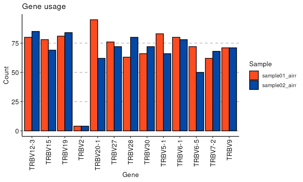
CDR3 analysis
Section titled “CDR3 analysis”The CDR3 region is the most variable part of the TCR. It spans the V-D-J junction and makes the most contacts with the peptide in the peptide-MHC complex. CDR3 sequence largely determines antigen specificity.
Key CDR3 properties:
- Length distribution: TCR beta CDR3 is typically 12 to 16 amino acids. The distribution is narrower than BCR heavy chain CDR3. CDR3 length affects which peptide-MHC complexes the TCR can bind.
- Amino acid composition: charge, hydrophobicity and specific residue preferences vary by V gene and by the antigen being recognised.
- Public CDR3 sequences: identical CDR3 sequences found in unrelated individuals. Public TCRs are far more common than public BCRs. They arise from biased V(D)J recombination and convergent selection by common pathogens.
Public TCR databases like VDJdb and McPAS-TCR catalog known TCR-antigen associations. If your expanded clonotypes match entries in these databases, you have candidate antigen assignments without any experimental validation.
The spectratype plot shows the length distribution directly. TCR beta CDR3s concentrate between twelve and seventeen amino acids, and both timepoints of the toy subject land in exactly that window:
# CDR3 amino acid length distributions per sample.sp1 <- as.data.frame(spectratype(imm$data[[1]], .col = "aa"))sp2 <- as.data.frame(spectratype(imm$data[[2]], .col = "aa"))sp1$Sample <- "day 0"sp2$Sample <- "day 28"spectra <- rbind(sp1, sp2)p <- ggplot(spectra, aes(factor(Length), Val, fill = Sample)) + geom_col(position = "dodge") + labs(x = "CDR3 length, amino acids", y = "Sequences")ggsave( "outputs/cdr3-lengths.png", p, width = 7, height = 4, dpi = 130, bg = "white")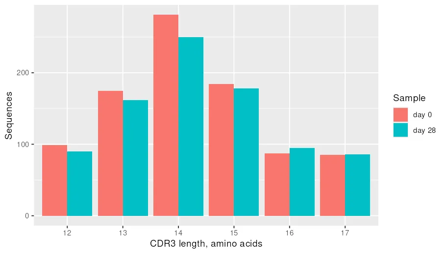
Clonal analysis
Section titled “Clonal analysis”A clonotype is defined by its CDR3 sequence and V/J gene usage. T cells sharing the same clonotype descended from the same V(D)J recombination event.
Clonal expansion
Section titled “Clonal expansion”Clonal expansion occurs when a T cell recognises antigen and proliferates. In sequencing data, expanded clones appear as groups of many sequences with identical CDR3 regions.
Key metrics:
- Clone size distribution: plot as a rank-abundance curve. Most clonotypes appear once. A few dominate.
- Top clone fraction: the percentage of the repertoire occupied by the largest clone. Values above 5% indicate strong expansion.
- Clonality index: 1 minus the normalised Shannon entropy. Ranges from 0 (perfectly even) to 1 (single clone dominates). Also called the productive clonality in the Adaptive immunoSEQ framework.
- Gini index: measures inequality in clone sizes. Near 0 means all clones are equal size. Near 1 means a few clones dominate.
Clonal expansion is expected during active infection, after vaccination and in the tumour microenvironment. In T cell lymphomas, a single malignant clone can dominate the entire repertoire.
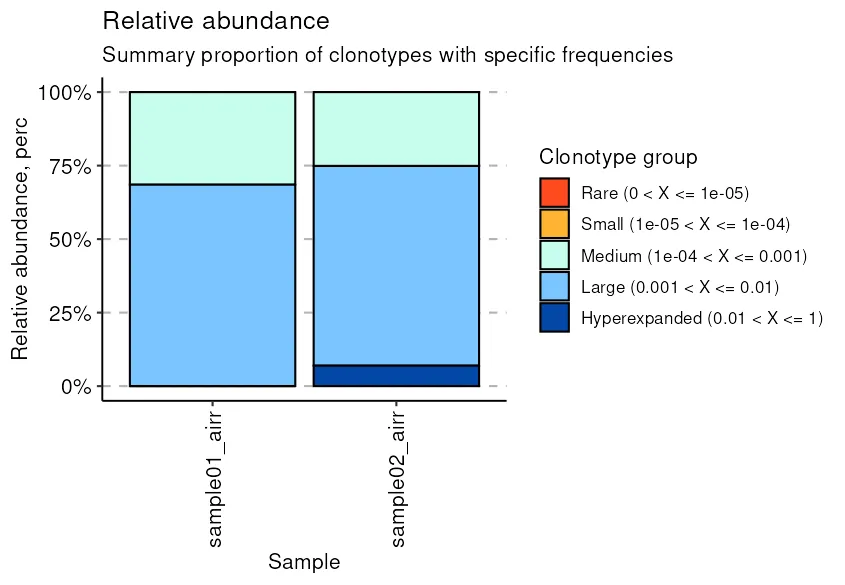
Two immunarch calls put numbers behind those metrics on the toy subject. The top-clone table shows what share of the repertoire each rank class holds, and the clonal-space plot bins every sequence by clone size:
# Share of the repertoire held by ranked clone groups.rc <- repClonality(imm$data, .method = "top")ggsave(  "outputs/top-clones.png",  vis(rc),  width = 5.5, height = 4.5, dpi = 130, bg = "white")
# Repertoire space held by each expanded-clone category.cs <- repClonality(imm$data, .method = "homeo")ggsave(  "outputs/clonal-space.png",  vis(cs),  width = 6.5, height = 4.5, dpi = 130, bg = "white")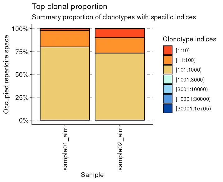
Tracking clones across samples
Section titled “Tracking clones across samples”A major advantage of TCR sequencing is longitudinal clonal tracking. Because TCR sequences are fixed and do not mutate, you can track the exact same clone across timepoints.
Common tracking analyses:
- Pre/post vaccination: which clones expand after vaccination? Do they persist at later timepoints?
- Tumour vs blood: which TIL clones are also found in peripheral blood? These could serve as liquid biopsy biomarkers.
- Treatment response: which clones expand or contract during immunotherapy?
The toy subject makes the tracking plot small enough to read at a glance. Four clonotypes, three of them real VDJdb records, all rise by roughly an order of magnitude between the two timepoints:
# Follow four clonotypes across both timepoints.tracked <- trackClonotypes( imm$data, c( "CASSLAPGATNEKLFF", "CAASTGIYGYTF", "CAGGTGETSPGELFF", "CAAGTRTDTQYF" ), .col = "aa")tracked_df <- as.data.frame(tracked)names(tracked_df)[1] <- "cdr3"long_df <- data.frame( cdr3 = rep(tracked_df$cdr3, 2), timepoint = rep(c("day 0", "day 28"), each = nrow(tracked_df)), proportion = c(tracked_df[[2]], tracked_df[[3]]))p <- ggplot(long_df, aes(timepoint, proportion, group = cdr3)) + geom_line() + geom_point(aes(color = cdr3), size = 2.5) + labs(x = NULL, y = "Fraction of repertoire", color = "CDR3")ggsave( "outputs/tracked-clones.png", p, width = 7, height = 4.5, dpi = 130, bg = "white")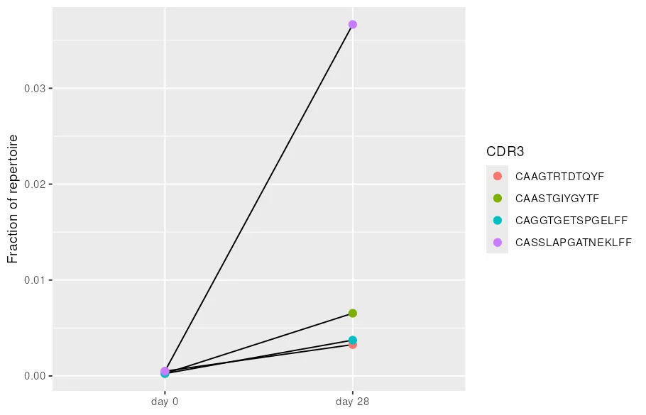
Diversity metrics
Section titled “Diversity metrics”Repertoire diversity measures how varied the T cell pool is. The same metrics used for BCR analysis apply to TCR data.
Common metrics
Section titled “Common metrics”- Richness: total number of unique clonotypes. Sensitive to sequencing depth.
- Shannon index: accounts for both the number of clonotypes and their relative abundance.
- Simpson index: the probability that two randomly chosen sequences belong to different clones. Less sensitive to rare clonotypes.
- Hill diversity profiles: a family of indices parameterised by q. Plotting across q values gives a complete picture from richness-weighted to evenness-weighted diversity.
On the toy subject the Hill profile is the clearest picture of what vaccination did. Day zero holds a broad repertoire whose effective size barely moves with q; day twenty-eight starts lower and collapses towards the handful of expanded clones as q grows:
# Diversity as a function of the order parameter q.dv <- repDiversity(imm$data, .method = "hill")ggsave( "outputs/hill-diversity.png", vis(dv), width = 7, height = 4.5, dpi = 130, bg = "white")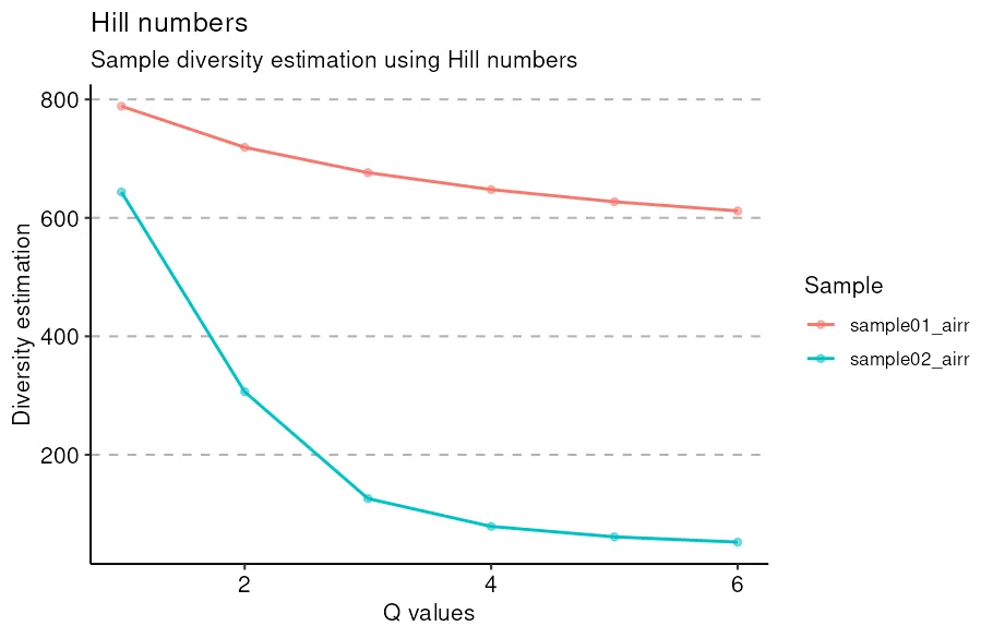
Rarefaction
Section titled “Rarefaction”Sequencing depth affects diversity estimates. Always compare diversity between samples at the same rarefied depth.
Rarefaction curves subsample to equal depth and recalculate diversity. If the curve has plateaued, you have captured most of the diversity. If it is still rising, deeper sequencing would find more clonotypes.
Antigen specificity prediction
Section titled “Antigen specificity prediction”This is where TCR analysis goes beyond what BCR analysis can currently offer. Computational tools can predict what antigen a TCR recognises based on its CDR3 sequence. This emerging field connects repertoire sequencing to functional immunology.
Why specificity prediction works for TCRs
Section titled “Why specificity prediction works for TCRs”TCRs with similar CDR3 sequences often recognise the same peptide-MHC complex. This is because the CDR3 loop makes direct contact with the peptide. Structurally similar CDR3 loops bind similar peptides. This principle of TCR convergence enables sequence-based prediction of specificity.
BCR specificity prediction is harder because antibodies use all six CDR loops to bind antigen and somatic hypermutation continuously changes the binding surface. TCR specificity is more concentrated in CDR3, and the sequence is fixed after thymic selection.
Reference databases
Section titled “Reference databases”Prediction tools rely on databases of experimentally validated TCR-antigen pairs.
| Database | Contents | Access |
|---|---|---|
| VDJdb | Curated TCR-peptide-MHC associations from literature | vdjdb.cdr3.net |
| McPAS-TCR | Pathology-associated TCR sequences | friedmanlab.weizmann.ac.il/McPAS-TCR |
| IEDB | Immune epitope database with some TCR annotations | iedb.org |
| 10x Genomics datasets | Public single-cell V(D)J datasets | 10xgenomics.com/datasets |
| PIRD | Pan immune repertoire database | db.cngb.org/pird |
VDJdb is the most widely used. It contains tens of thousands of TCR-peptide-MHC triplets. Most entries are for viral epitopes from CMV, EBV, influenza and SARS-CoV-2.
Clustering-based methods
Section titled “Clustering-based methods”These tools group TCRs by CDR3 similarity and look for clusters enriched for a specific antigen.
GLIPH2 (Grouping of Lymphocyte Interactions by Paratope Hotspots) identifies TCR specificity groups by finding shared CDR3 motifs. It looks for short amino acid patterns of 2 to 4 residues that are statistically enriched compared to a background repertoire. TCRs sharing a motif are grouped into a specificity cluster. GLIPH2 can process large datasets and does not require pre-existing antigen labels.
# Example GLIPH2 input: tab-separated CDR3b and TRBV gene# CDR3b TRBV patient_id# CASSLAPGATNEKLFF TRBV5-1 patient01# CASSYSRGSGANVLTF TRBV6-1 patient01TCRdist3 calculates a distance metric between TCRs based on CDR1, CDR2 and CDR3 amino acid similarity. It uses a substitution matrix trained on TCR structural data. TCRs below a distance threshold are grouped into neighbourhoods. TCRdist3 can identify convergent TCR responses across individuals and map them to known epitopes.
ClusTCR uses the Faiss library to perform fast, approximate clustering of millions of CDR3 sequences. It is designed for large-scale repertoire datasets where pairwise distance calculations are computationally prohibitive.
Deep learning methods
Section titled “Deep learning methods”Machine learning models trained on TCR-antigen binding data can predict specificity for individual TCR sequences.
DeepTCR is a deep learning framework for TCR repertoire analysis. It uses convolutional neural networks to learn sequence features from CDR3 and V gene usage. DeepTCR can classify TCR repertoires by disease state and predict antigen specificity at the single-sequence level.
ERGO-II predicts whether a given TCR-peptide pair will bind. It takes a CDR3 beta sequence and a peptide sequence as input and returns a binding probability. ERGO-II uses autoencoder-based representations of both the TCR and the peptide. It was trained on VDJdb data and performs best on epitopes well represented in the training set.
NetTCR-2.1 predicts TCR-peptide binding for specific HLA alleles. It uses convolutional neural networks trained on peptide-MHC tetramer sorting data. NetTCR is epitope-specific: you train or select a model for each target peptide-MHC combination.
pMTnet predicts TCR binding to peptide-MHC class I complexes. It can handle novel peptides not seen during training by using a transfer learning approach from protein structure. pMTnet is particularly useful for predicting T cell recognition of tumour neoantigens.
TITAN (TCR Interaction with Transformer Attention Networks) uses attention-based neural networks to predict TCR-epitope binding. The attention mechanism highlights which CDR3 positions are most important for binding each specific peptide.
Practical considerations
Section titled “Practical considerations”Key limitations to keep in mind:
- Training data bias: most validated TCR-antigen pairs come from a handful of immunodominant viral epitopes. Predictions for understudied epitopes are less accurate.
- MHC restriction: specificity depends on both the peptide and the MHC allele. Most tools require MHC information for accurate predictions. Some tools like ERGO-II work without it but have lower accuracy.
- Paired chain information: the alpha chain contributes to specificity. Tools using only the beta chain CDR3 miss this contribution. Paired alpha-beta data improves predictions.
- Validation: experimentally confirm computational predictions using peptide-MHC tetramers, ELISPOT or functional killing assays.
Tools overview
Section titled “Tools overview”| Tool | Purpose | Input |
|---|---|---|
| IgBLAST | V(D)J assignment | FASTA sequences |
| MiXCR | V(D)J assignment and clonotype assembly | FASTQ files |
| immunarch (R) | Repertoire analysis, diversity, gene usage | AIRR tables, immunoSEQ output |
| Scirpy (Python) | Single-cell TCR analysis with Scanpy | AnnData objects |
| GLIPH2 | Specificity group clustering | CDR3 + V gene tables |
| TCRdist3 | Distance-based clustering | CDR3 + V/J genes |
| ClusTCR | Fast large-scale CDR3 clustering | CDR3 sequences |
| DeepTCR | Deep learning repertoire classification | CDR3 + V gene, optional HLA |
| ERGO-II | TCR-peptide binding prediction | CDR3 + peptide sequences |
| NetTCR-2.1 | Epitope-specific binding prediction | CDR3 + peptide + HLA |
| pMTnet | Pan-peptide binding prediction | CDR3 + peptide-MHC |
| TITAN | Attention-based binding prediction | CDR3 + peptide sequences |
Summary
Section titled “Summary”- V(D)J assignment with IgBLAST or MiXCR identifies germline gene usage and CDR3 sequences.
- V gene usage and CDR3 properties describe the composition of the T cell repertoire.
- Clonal expansion analysis identifies antigen-driven T cell responses. Clones can be tracked longitudinally because TCR sequences do not mutate.
- Diversity metrics quantify how broad or focused the repertoire is. Always account for sequencing depth with rarefaction.
- Antigen specificity prediction uses CDR3 sequence similarity and deep learning to predict what a TCR recognises. Tools like GLIPH2, TCRdist3, DeepTCR, ERGO-II and pMTnet connect sequence data to function.
- Reference databases like VDJdb and McPAS-TCR provide experimentally validated TCR-antigen associations for comparison.