Running nf-core/airrflow for TCR

nf-core/airrflow processes both BCR and TCR sequencing data. The same pipeline handles both receptor types. You select TCR mode through the samplesheet and parameters. This page covers the TCR-specific considerations and then works through the downstream analyses the BCR page leaves out: repertoire analysis with immunarch, single-cell clonotypes with scirpy, and antigen matching against VDJdb.

airrflow for TCR vs BCR

The pipeline architecture is identical for both receptor types. pRESTO handles read preprocessing, IgBLAST performs V(D)J annotation and Change-O parses the output. The key differences are:

Aspect	BCR mode	TCR mode
pcr_target_locus	ig	tr
Reference database	IMGT immunoglobulin genes	IMGT T cell receptor genes
Somatic hypermutation	Analysed	Not relevant
Clonal threshold	Gaussian mixture model	Simpler, less variation
Isotype analysis	Yes (IgM, IgG, IgA, IgE)	No (only TRBC1/TRBC2)

IgBLAST automatically uses the correct germline database based on the locus setting. You do not need to specify the reference database separately.

Input samplesheet

The samplesheet format is the same as for BCR. The critical field is pcr_target_locus, which must be set to tr for TCR data.

sample_id,filename_R1,filename_R2,subject_id,species,tissue,pcr_target_locus,treatment,collection_time_point_relative
sample01,sample01_R1.fastq.gz,sample01_R2.fastq.gz,subject01,human,blood,tr,none,0
sample02,sample02_R1.fastq.gz,sample02_R2.fastq.gz,subject01,human,blood,tr,anti-PD1,28
sample03,sample03_R1.fastq.gz,sample03_R2.fastq.gz,subject02,human,tumour,tr,none,0

You can mix BCR and TCR samples in the same samplesheet. The pipeline processes each locus separately with the appropriate reference database.

Caution

If you accidentally set pcr_target_locus to ig for TCR data, IgBLAST will try to align your sequences against immunoglobulin genes. Most sequences will fail annotation or receive incorrect assignments. Always double-check this field.

Key parameters

The same --library_generation_method parameter controls the preprocessing workflow. Common values for TCR data:

Value	Protocol
specific_pcr_umi	Multiplex PCR with UMIs
race_uid	5’RACE with UMIs
specific_pcr	Multiplex PCR without UMIs
dt_5p_race	5’RACE with template switching

Other key parameters:

• --umi_length: length of the UMI. Protocol-dependent, typically 12 or 15.
• --vprimers: FASTA file with V gene primer sequences. These must be TCR V gene primers, not BCR primers.
• --cprimers: FASTA file with constant region primer sequences. For TCR beta, these target TRBC1 and TRBC2.

Example command

Running airrflow on a TCR multiplex PCR dataset with UMIs:

nextflow run nf-core/airrflow \
  -r 5.1.0 \
  -profile podman \
  --input samplesheet.csv \
  --library_generation_method specific_pcr_umi \
  --umi_length 12 \
  --vprimers tcr_vprimers.fasta \
  --cprimers tcr_cprimers.fasta \
  --outdir results

For running on AWS Batch:

nextflow run nf-core/airrflow \
  -r 5.1.0 \
  -profile awsbatch \
  --input s3://mybucket/samplesheet.csv \
  --library_generation_method specific_pcr_umi \
  --umi_length 12 \
  --vprimers s3://mybucket/tcr_vprimers.fasta \
  --cprimers s3://mybucket/tcr_cprimers.fasta \
  --outdir s3://mybucket/results \
  -work-dir s3://mybucket/work

Pipeline steps for TCR data

The four stages are the same as for BCR data with minor differences.

1. pRESTO: read preprocessing

pRESTO processing is identical for TCR and BCR. UMI extraction, consensus building, primer masking and paired-end assembly all work the same way. The only difference is the primer sequences you provide.

2. IgBLAST: V(D)J annotation

IgBLAST uses the IMGT TCR germline database instead of the immunoglobulin database. It identifies TRBV, TRBD and TRBJ genes for the beta chain, or TRAV and TRAJ genes for the alpha chain.

The annotation output includes:

• V, D and J gene assignments (for example TRBV6-1, TRBD1, TRBJ2-1)
• CDR3 nucleotide and amino acid sequence
• Framework and CDR region boundaries
• Productive vs non-productive rearrangement status

3. Change-O: parsing and filtering

Change-O parses the IgBLAST output into AIRR format. For TCR data, the mutation frequency columns will show near-zero values because TCRs do not undergo somatic hypermutation. This is expected.

The clonal distance threshold calculation works the same way, fitting a Gaussian mixture model to nearest-neighbour CDR3 distances. For TCR data, the distribution tends to be cleaner because there is no somatic hypermutation blurring the boundary between clonal and non-clonal sequences.

4. Clonal assignment

Sequences are grouped into clonotypes based on shared V gene, J gene and similar CDR3 sequence. The threshold from step 3 determines what counts as similar enough.

For TCR data, clonal assignment is more straightforward than for BCR. Without somatic hypermutation, members of a true clone have identical or near-identical CDR3 sequences. The within-clone variation comes primarily from sequencing errors rather than biological mutation.

Output structure

The results directory has the same structure as BCR output:

results/
├── presto/            # pRESTO preprocessing logs and stats
├── igblast/           # Raw IgBLAST output
├── changeo/           # Parsed AIRR tables, threshold plots
├── clonal_analysis/   # Clone assignments
├── repertoire_analysis/ # Gene usage, diversity plots
├── multiqc/           # Summary report
└── pipeline_info/     # Execution logs and resource usage

The AIRR-formatted TSV files in changeo/ are the main output. For TCR data, the locus column will contain TRB or TRA. The v_call, d_call and j_call columns will contain TRBV/TRBD/TRBJ gene names instead of IGHV/IGHD/IGHJ.

Note

As on the BCR page, the Nextflow commands above show how a real analysis starts and are not executed here. The worked examples below do run in this site’s container. They use three committed fixtures shaped like airrflow output: two AIRR tables for one toy subject before and after a vaccination, a synthetic 10x V(D)J contig table from one tumour biopsy, and a small real excerpt of the VDJdb database. Three of the expanded clonotypes in the toy subject are real VDJdb records, so the antigen-matching example finds something true.

Repertoire analysis with immunarch

The immunarch package is the broadest R toolkit for repertoire analysis, and it reads AIRR-format tables directly. Loading the two timepoints needs no conversion step:

library(immunarch)

# Two AIRR tables airrflow writes into changeo/, t0 and t28.
imm <- repLoad(c("sample01_airr.tsv", "sample02_airr.tsv"))

# V gene usage per sample.
gu <- geneUsage(imm$data, .gene = "hs.trbv")
print(gu)

# True diversity of each timepoint.
div <- repDiversity(imm$data, .method = "div")
print(div)

# Fraction of the repertoire held by the top clones.
rc <- repClonality(imm$data, .method = "top")
print(round(rc, 4))

# A tibble: 13 × 3
   Names    sample01_airr sample02_airr
   <chr>            <int>         <int>
 1 TRBV12-3            80            85
 2 TRBV15              78            69
 3 TRBV19              81            84
 4 TRBV2                4             4
 5 TRBV20-1            95            62
 6 TRBV27              76            72
 7 TRBV28              63            80
 8 TRBV30              66            72
 9 TRBV5-1             83            66
10 TRBV6-1             80            78
11 TRBV6-5             72            50
12 TRBV7-2             62            68
13 TRBV9               71            71
         Sample     Value
1 sample01_airr 627.20467
2 sample02_airr  61.32853
                  10    100 1000 3000 10000 30000 1e+05
sample01_airr 0.0200 0.2000    1    1     1     1     1
sample02_airr 0.0994 0.2675    1    1     1     1     1
attr(,"class")
[1] "immunr_top_prop" "matrix"          "array"

The usage table shows every TRBV gene detected in either sample, with one column per sample. Diversity collapses the picture to one number per sample, and it falls by an order of magnitude after vaccination: the response narrowed onto a few clones. The clonality table says the same thing from the other side. The top 10 clonotypes hold 2% of the repertoire at day 0 and close to 10% at day 28.

Because TCR sequences do not mutate, you can go one step further and follow individual clonotypes across the timepoints:

# Follow the expanded clones across both timepoints.
tracked <- trackClonotypes(
  imm$data,
  c(
    "CASSLAPGATNEKLFF", "CAASTGIYGYTF",
    "CAGGTGETSPGELFF", "CAAGTRTDTQYF"
  ),
  .col = "aa"
)
tracked_df <- as.data.frame(tracked)
tracked_df[, -1] <- round(tracked_df[, -1], 4)
print(tracked_df)

           CDR3.aa sample01_airr sample02_airr
1     CAAGTRTDTQYF         5e-04        0.0033
2     CAASTGIYGYTF         2e-04        0.0065
3  CAGGTGETSPGELFF         2e-04        0.0037
4 CASSLAPGATNEKLFF         5e-04        0.0366

Each row is one clonotype and each column one sample. Every clone here grows by roughly an order of magnitude, which is what a vaccine response looks like in this kind of table. Three of the four rows are real CMV, EBV and influenza-specific receptors recorded in VDJdb; that connection is made explicit further down this page.

Single-cell clonotypes with scirpy

Bulk sequencing tells you a clonotype expanded. Single-cell sequencing adds chain pairing and phenotype. scirpy brings 10x Genomics V(D)J data into the scanpy world:

import matplotlib.pyplot as plt
import scirpy as ir

# A 10x Genomics V(D)J contig table from one tumour biopsy.
adata = ir.io.read_10x_vdj("filtered_contig_annotations.csv")

ir.tl.chain_qc(adata)
print(adata.obs["chain_pairing"].value_counts().to_string())

# Group receptors whose beta CDR3s sit within alignment distance.
ir.pp.ir_dist(adata, metric="alignment", sequence="aa")
ir.tl.define_clonotype_clusters(
    adata,
    sequence="aa",
    metric="alignment",
    receptor_arms="VDJ",
    dual_ir="primary_only",
)
clusters = adata.obs["cc_aa_alignment"]
print(f"{clusters.nunique()} clonotype clusters")
print(clusters.value_counts().head().to_string())

# Expansion bins over those clusters.
ir.tl.clonal_expansion(adata, target_col="cc_aa_alignment")
print(adata.obs["clonal_expansion"].value_counts().to_string())

chain_pairing
orphan VDJ     39
single pair    21
50 clonotype clusters
cc_aa_alignment
0    6
1    4
2    3
3    1
4    1
clonal_expansion
<= 1    47
> 2     13
<= 2     0
nan      0

Two definitions matter here. A strict clonotype requires identical CDR3 nucleotide sequences. A clonotype cluster groups receptors whose amino acid CDR3s are similar under a distance metric, which is how convergent responses get recognised. With the beta arm alone, sixty cells collapse into fifty clusters, and three clusters hold six, four and three cells respectively. Those are the expanded tumour-infiltrating clones.

The expansion call bins cells by their cluster size, and the plot splits the bins by chain pairing status:

import matplotlib.pyplot as plt
import scirpy as ir

fig, ax = plt.subplots(figsize=(4, 3))
ir.pl.clonal_expansion(
    adata,
    target_col="cc_aa_alignment",
    groupby="chain_pairing",
    ax=ax,
)
fig.savefig("outputs/scirpy-clonal-expansion.png", dpi=150, bbox_inches="tight")
print("saved outputs/scirpy-clonal-expansion.png")

saved outputs/scirpy-clonal-expansion.png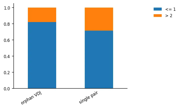

Antigen specificity prediction

Feed the AIRR output into specificity prediction tools.

GLIPH2 requires a simple table of CDR3 beta sequences and TRBV genes:

import pandas as pd

airr_df = pd.read_csv("sample01_airr.tsv", sep="\t")

# GLIPH2 reads a table of CDR3 beta sequences and V genes.
gliph_input = airr_df[["junction_aa", "v_call"]].copy()
gliph_input.columns = ["CDR3b", "TRBV"]
print(gliph_input.head(5).to_string(index=False))

           CDR3b     TRBV
CASSLAPGATNEKLFF  TRBV5-1
  CASSYSGTNEKLFF   TRBV19
CASSDRGGYEQYFGPG TRBV20-1
  CASSQETGNYGYTF  TRBV6-5
  CASSIGGSYNEQFF   TRBV28

For a multi-subject study you would add a patient column; GLIPH2 uses it to separate public motifs from private ones.

VDJdb matching identifies known antigen associations. Exact CDR3 matches are the conservative form of annotation: no similarity threshold, no model, just a lookup. The committed excerpt holds 184 high-confidence human TRB records for four common epitopes, NLVPMVATV from CMV, GILGFVFTL from influenza, GLCTLVAML from EBV and SLLMWITQV from HTLV-1:

import pandas as pd

vdjdb = pd.read_csv("vdjdb_excerpt.txt", sep="\t")
airr_df = pd.read_csv("sample01_airr.tsv", sep="\t")

matches = airr_df.merge(
    vdjdb[["cdr3", "antigen.epitope", "antigen.gene"]],
    left_on="junction_aa",
    right_on="cdr3",
    how="inner",
)
print(f"{len(matches)} sequences match a known antigen association")
print(
    matches[["junction_aa", "v_call", "antigen.epitope"]]
    .drop_duplicates()
    .to_string(index=False)
)

3 sequences match a known antigen association
    junction_aa v_call antigen.epitope
   CAASTGIYGYTF TRBV19       GILGFVFTL
CAGGTGETSPGELFF  TRBV2       GLCTLVAML
   CAAGTRTDTQYF  TRBV2       NLVPMVATV

Three sequences hit, and three of the four clonotypes the tracking example followed are among them: the influenza M1, EBV BMLF1 and CMV pp65 receptors. A merge like this turns an anonymous expanded clone into a hypothesis you can take to the bench. In a real repertoire of a million sequences the same lookup takes seconds; the interpretation stays the same.

Common issues

Wrong pcr_target_locus. Setting this to ig instead of tr is the most common mistake. IgBLAST will fail to annotate most sequences or assign incorrect immunoglobulin genes. Always verify this field in your samplesheet.

TCR-specific primer files. Make sure your --vprimers and --cprimers FASTA files contain TCR primers, not BCR primers. Using BCR primers will cause pRESTO to fail at the primer masking step.

Low clonal diversity threshold. TCR data tends to have sharper clonal boundaries than BCR data because there is no somatic hypermutation. If the Gaussian mixture model sets an unusually low threshold, check whether your data has sufficient depth. Small datasets may not provide enough pairs for reliable threshold estimation.

Alpha chain dual rearrangements. If you are sequencing the alpha chain, remember that a single T cell can have two productive alpha chain rearrangements. This means you cannot assume a one-to-one relationship between alpha chain sequences and cells in bulk sequencing data.

Memory for clonal assignment. As with BCR, the clonal assignment step loads all sequences from one subject into memory. For deep sequencing experiments with millions of sequences per subject, this can exceed available RAM.

Summary

• nf-core/airrflow processes TCR data with the same pipeline as BCR data. Set pcr_target_locus to tr in the samplesheet.
• The --library_generation_method parameter must match your library preparation protocol.
• IgBLAST automatically uses the IMGT TCR germline database when the locus is set to tr.
• Somatic hypermutation analysis is not relevant for TCR data. Near-zero mutation frequencies are expected.
• Clonal assignment is more straightforward for TCR than BCR because clone members have identical or near-identical CDR3 sequences.
• Downstream analysis with immunarch, scirpy, GLIPH2 or VDJdb matching connects sequence data to biological function.